Visualisation

Main Window

The main window on render will display a 3D view. The top menu bar allows the user to open additional 3D and 2D views which can also be closed. See Figure 32 and Figure 33.

3D Visualisation

There are five main components in the 3D view: the Top Menu, the Side Menu, the Main View, the Raytracer Toggle button, and the View Preset button. See Figure 34.

Main 3D view

The main 3D view provides interactive navigation of the model in 3D space. Users can rotate, pan and zoom to inspect the geometry from different perspectives.

Mouse Controls (Orbital and Orthographic)

• Rotate – Left-click and drag to rotate the camera around the model.

• Pan – Hold Shift, then left-click and drag to move the camera parallel to the model.

• Zoom – Use the mouse wheel to zoom in and out.

Mouse Controls (Flying)

• Rotate – Left-click and drag to change yaw (left/right) and pitch (up/down).

• Rotate – Hold Shift and move the mouse to rotate (same effect as left-click).

• Zoom – Use the mouse wheel to move the camera forward/backward.

Keyboard Controls (Orbital and Orthographic)

• Rotate – Use the arrow keys (←, →, ↑, ↓) to rotate the camera around the model.

• Pan – Hold Shift and use the arrow keys to pan the camera.

• Zoom – Press + or - to zoom in and out.

Keyboard Controls (Flying)

• Move – W / ↑ to move forward, S / ↓ to move backward.

• Move – A / ← to move left, D / → to move right.

• Rotate – Hold Shift + W / ↑ to pitch up.

• Rotate – Hold Shift + S / ↓ to pitch down.

• Rotate – Hold Shift + A / ← to yaw left.

• Rotate – Hold Shift + D / → to yaw right.

• Roll – Z to roll counterclockwise, C to roll clockwise.

• Zoom – Use the mouse wheel (no keyboard zoom binding).

Top Menus

The two main menus in this area are Edit Materials and Slice Model. The Edit Materials menu may appear under a different name depending on the current view type (for example, Edit Cells). See Figure 35.

Edit Materials

The Edit Materials button opens a drop-down menu listing all available materials, cells, and related items. From this menu the user can:

• Toggle individual items on or off.

• Switch items to wireframe mode.

• Change colours.

• Select and highlight multiple items at once to apply changes (such as turning them on or off) in a single action.

See Figure 36.

Slice Model

The Slice Model widget allows the user to cut through the model using an axis-aligned plane. As the slice value is adjusted a plane is displayed in the view to indicate the exact location of the cut. See Figure 37.

Side Menus

The Side Menu provides access to a range of utility functions. If the MCNP input includes tallies, points or meshes, these will also appear in the menu alongside the standard functions. See Figure 38.

Switch Views

The current view can be switched to display Cells, Materials, Universes, Densities, or Importances. Clicking on any of these options changes the active view accordingly. See Figure 39.

Utilities

The Utilities menu (see Figure 40) allows the user to:

• Toggle the axis and grid display on or off.

• Show or hide cell outlines.

• Run checks for overlapping or void regions within the model.

Open Contour Console

The Open Contour Console launches the contour console, where mesh tallies, particle track files and CAD files can be viewed. These functions are described in Sections 16.4, 16.4.2 and 16.4.3. See Figure 41.

Export

The Export option allows the user to save either the current screen image or the CAD view generated by the CAD processor[^2], see Figure 42.

Cameras

Cyclone provides three camera modes: Orthographic, Orbital, and Flying. In addition, a custom view can be defined by specifying both the camera position and the camera target (also known as the point of interest). See Figure 43.

Tallies, Points and Meshes

The following can be plotted:

• F4 tallies

• F5 Tallies

• F6 Tallies

• ADVANTG Mesh

• FMESH (rectilinear)

• KSRC points

• DXT Spheres

Context Menu

The context menu (Figure 44) brings up information about the current position that is visible. It displays the following data:

• Cell

• Material

• Surface

• Universe

• Density

• Importance

It also shows the 3D position in space. The user can centre the camera to target here and isolate the cell in the current view. The same features described in Section 16.2.2.1 are available, allowing the current cell to be toggled on or off, displayed in wireframe, or assigned a different colour.

Raytracer

The Raytracer button (Figure 45) toggles raytracing on and off. If the view has been opened in raytracer-only mode, this button remains permanently enabled.

When active, the raytracer begins with a coarse, pixelated image that progressively refines into a clearer view. If the camera is moved, Cyclone temporarily switches back to the CAD view for responsiveness. Once movement stops, the raytracer resumes and re-renders the scene.

Raytracing produces high-quality images and supports advanced visual effects such as transparency, reflection and refraction, see Figure 46.

Prefix Views

The Prefix button (Figure 47) expands to show 6 different views that align the image with the main axis, clicking on one of the views changes the position of the camera with respect to the model and the axis.

Settings

Clicking the Settings cog (Figure 48) opens the settings panel (Figure 49), where stylistic options for the current view can be adjusted. From here, the background colour can be changed, lighting configured, raytracer options modified and point colours for tallies set.

The full breakdown of options is shown in Table 5.

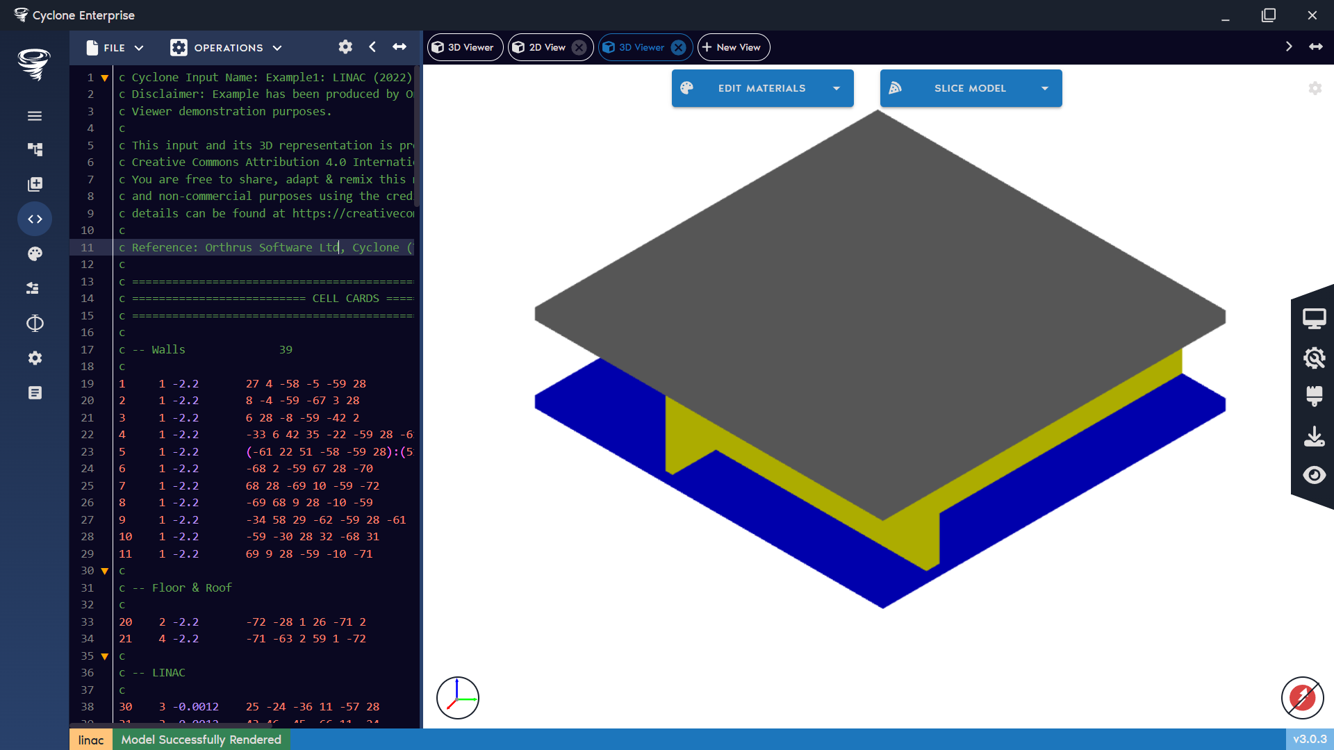
Figure 32: Main image view

Figure 33: Main view app bar

Figure 34: 3D view – main sections highlighted

Figure 35: 3D view – edit materials and slice model buttons

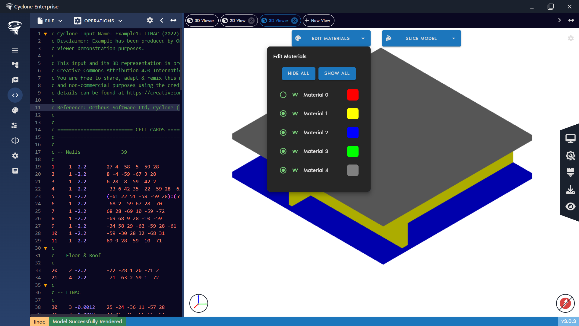
Figure 36: 3D view – edit materials menu

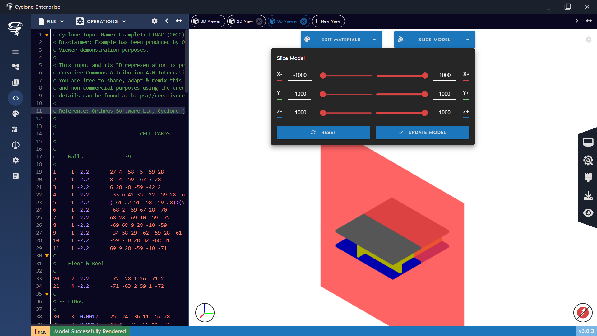
Figure 37: 3D view – slice model

Figure 38: 3D view – side menu

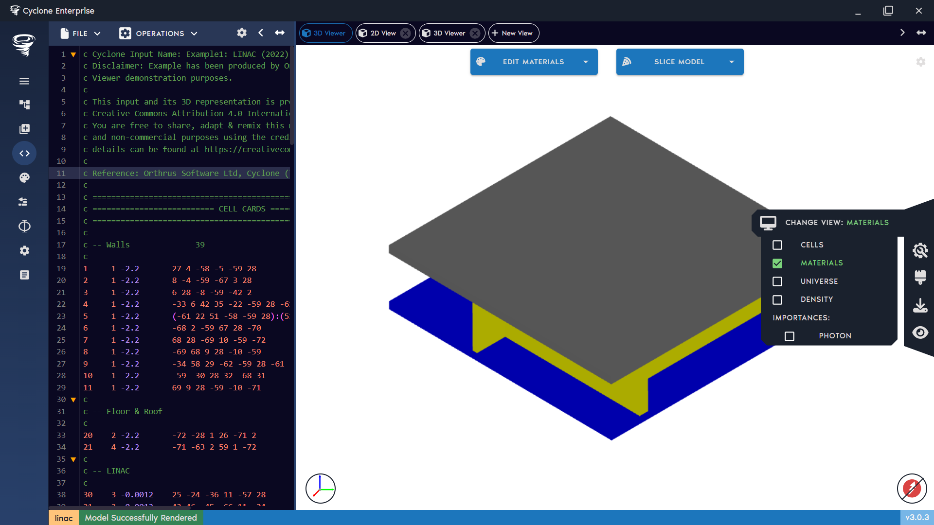
Figure 39: 3D view – change view preference

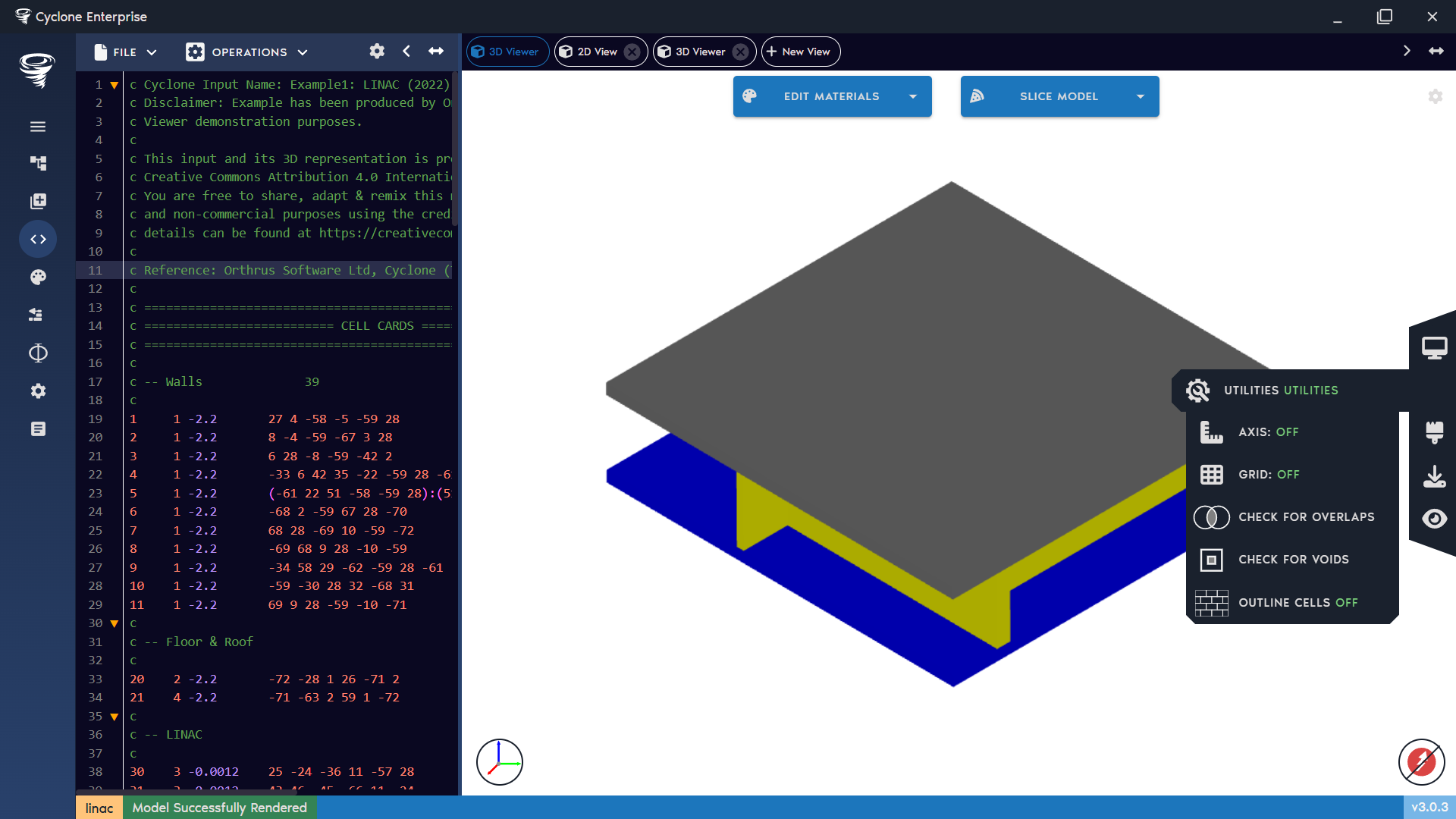
Figure 40: 3D view – select utilities

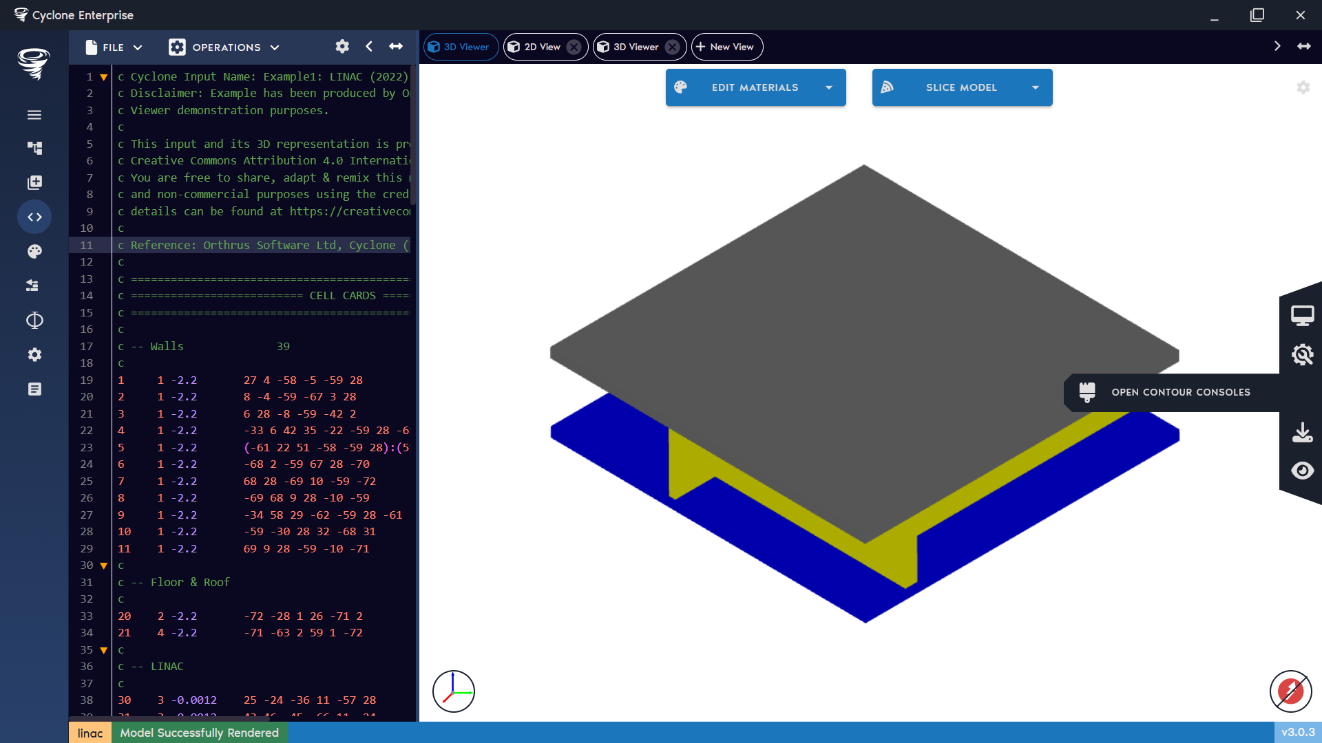
Figure 41: 3D view – open contour consoles

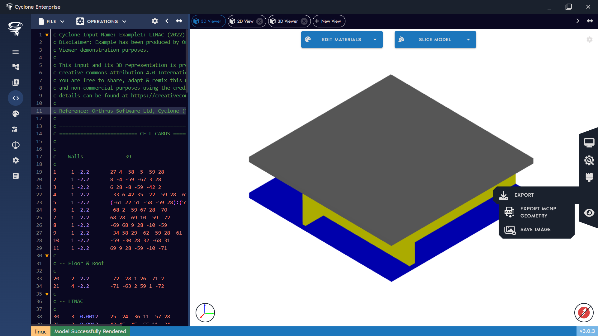
Figure 42: 3D view – export options

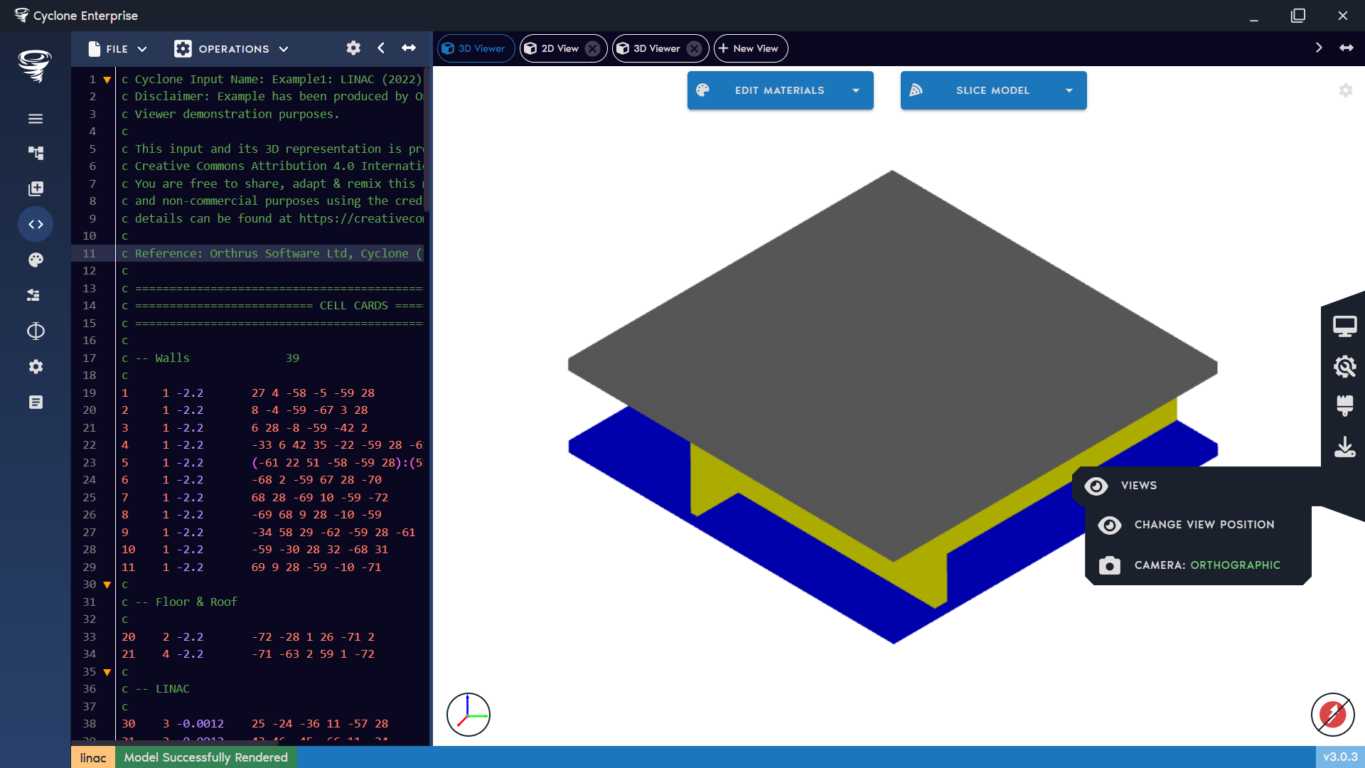
Figure 43: 3D view – modify view

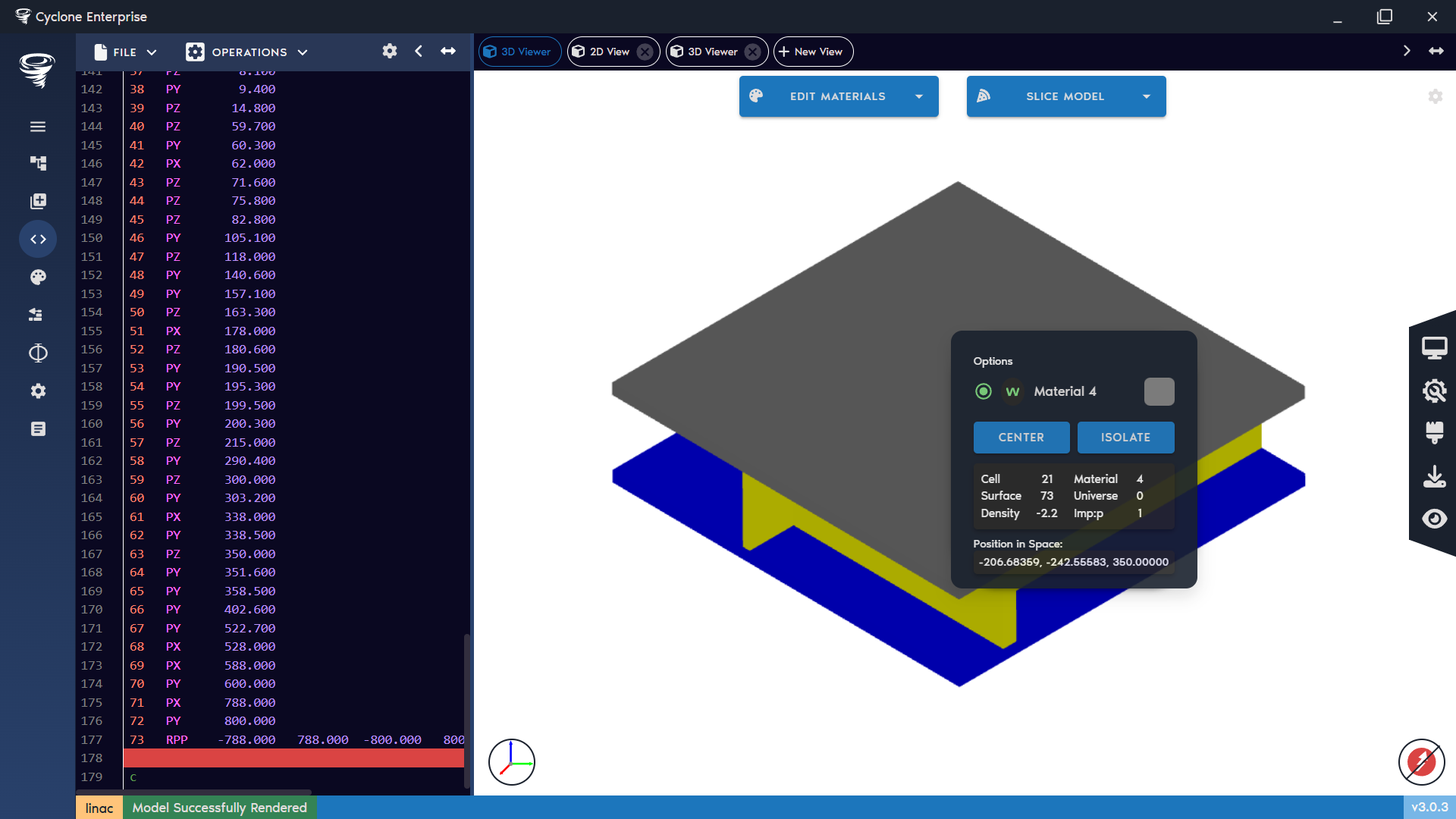
Figure 44: 3D view – context menu

Figure 45: 3D view – raytracer button

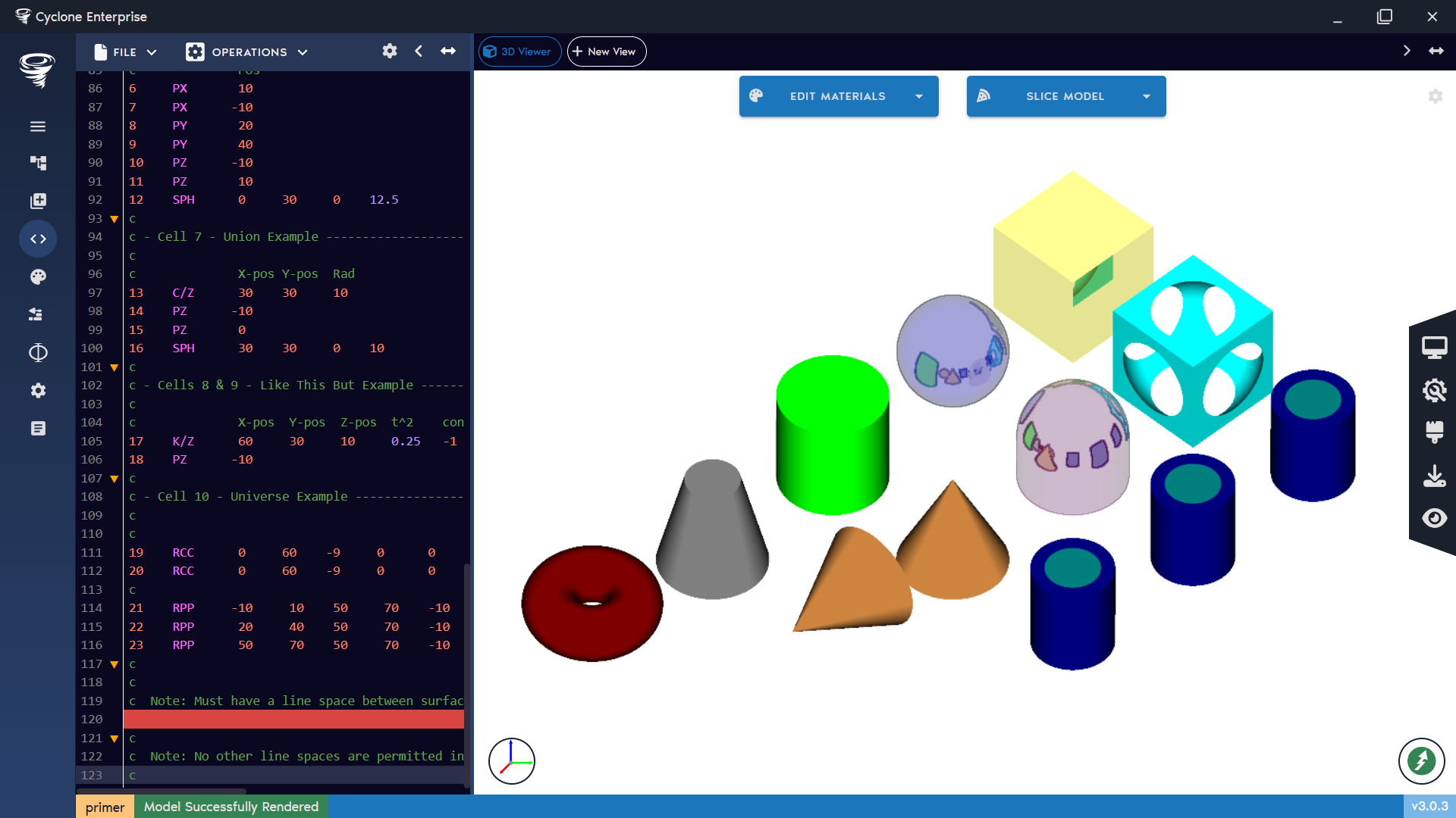
Figure 46: 3D view – raytraced image

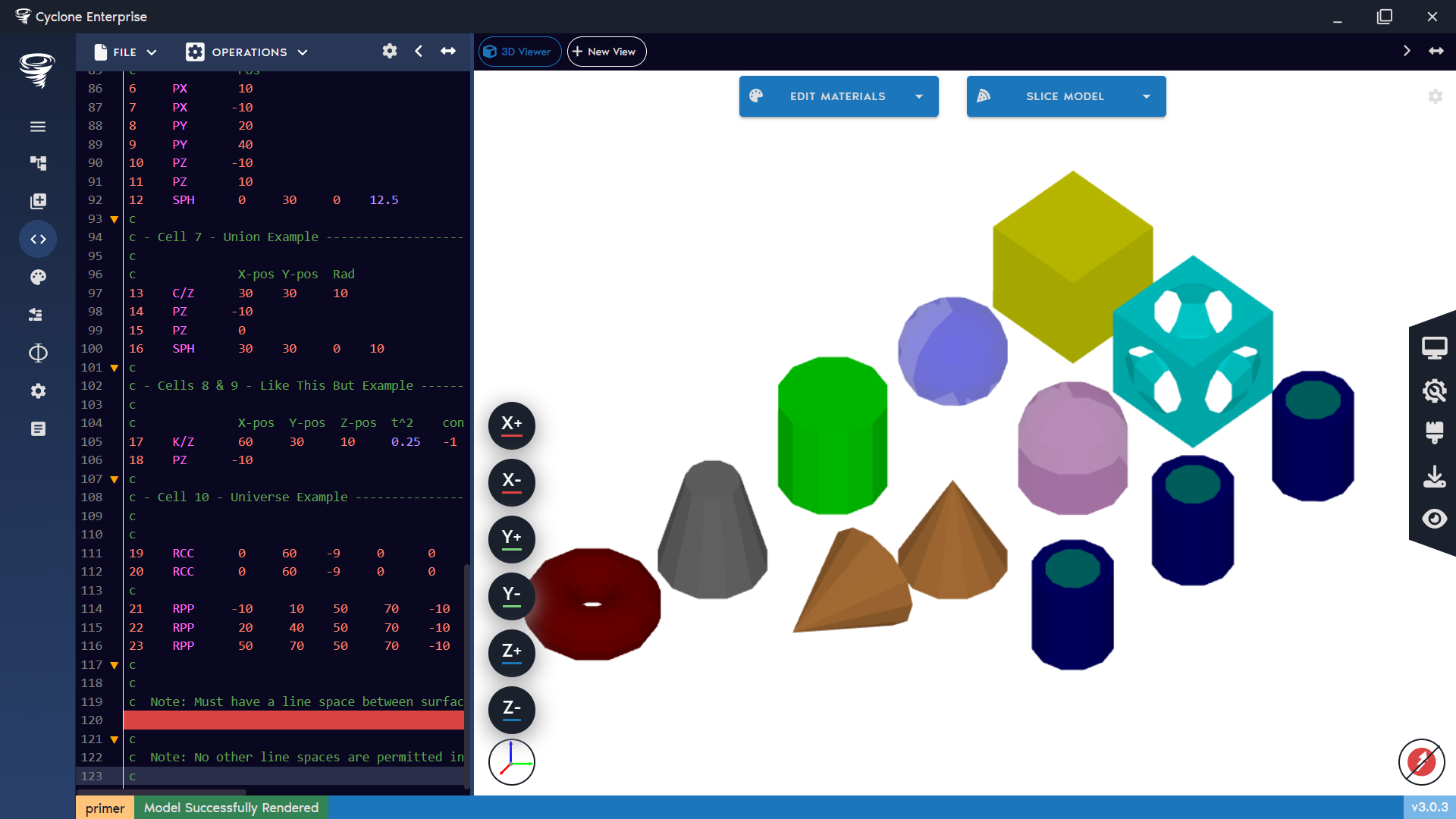
Figure 47: 3D view – preset camera views

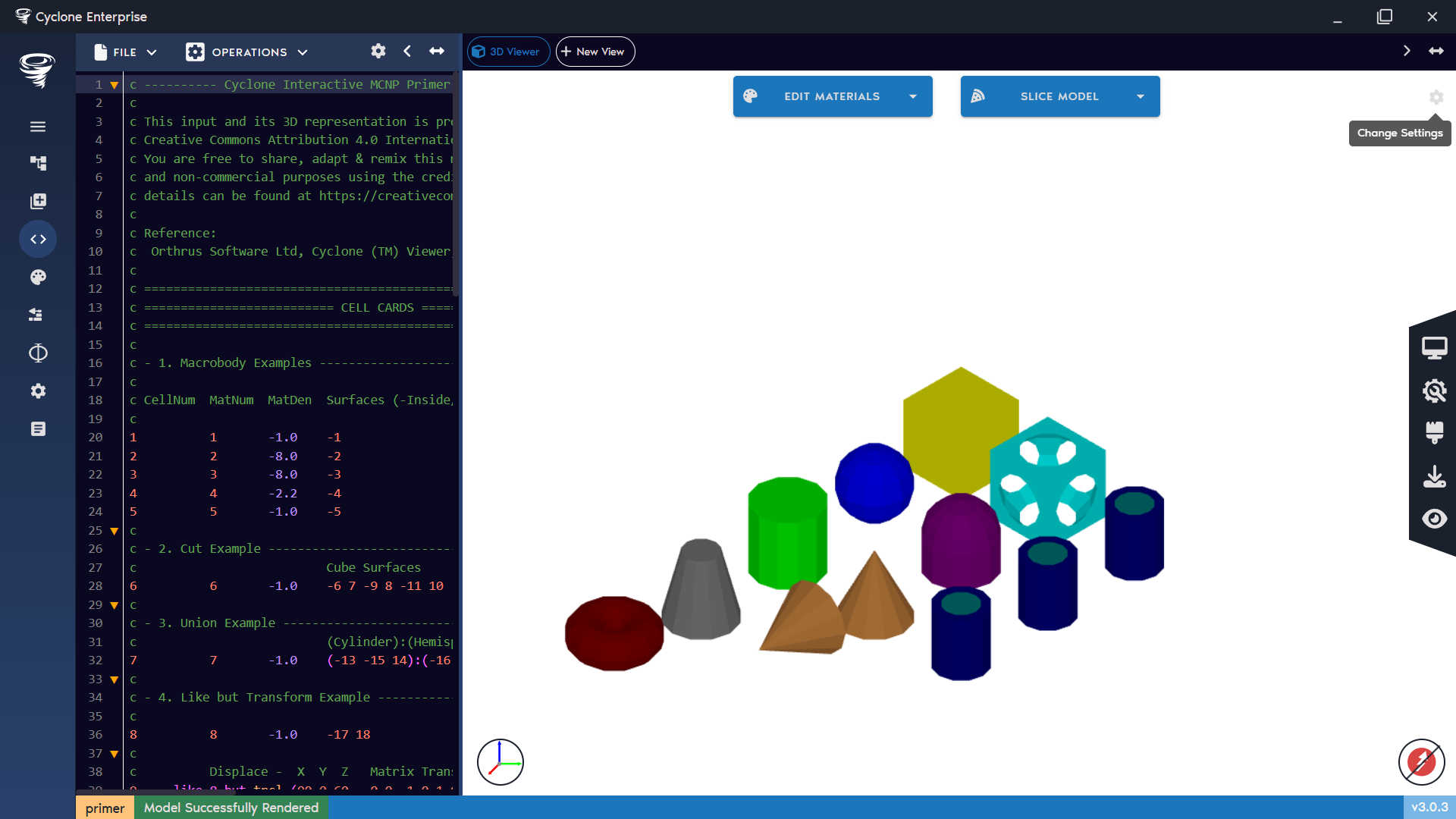
Figure 48: 3D view – settings button

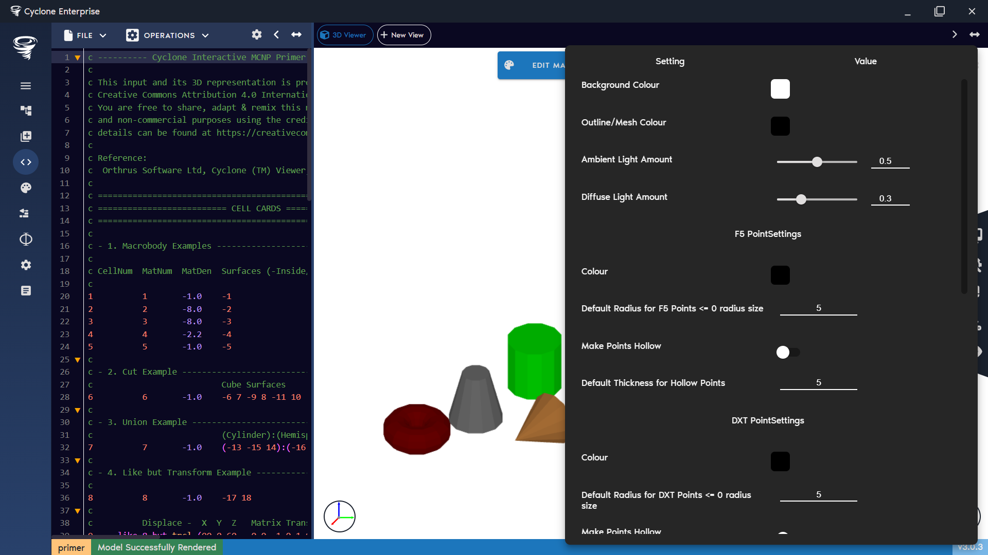
Figure 49: 3D view – settings menu

Table 5: Full list of 3D view settings

2D Visualisation

A 2D sliced view can be opened via the New View button at the top of the main 3D view (Figure 50) or via the Popout button (Figure 51).

Main 2D View

The main 2D view consists of three areas: the 2D slice display, the side menu options and the bottom view data. See Figure 52.

Raytracer Theory

The 2D View uses the raytracer exclusively and can operate in two modes:

1. Default Mode

   • Rays are cast into the model from left to right and from bottom to top across the screen.

   • The two resulting images are overlaid, and any differences between them are shown using the error colour.

   • This method is generally accurate, though small divergences may appear due to minute tolerances.

2. Full Raytracer “Find Me” Mode

   • For each pixel, the world-space 3D coordinate is calculated.

   • The raytracer’s “find me” function is then used to determine the correct position in space.

   • This method also relies on the first two ray directions to collect surface information.

   • It is more computationally intensive and therefore slower, but it avoids the tolerance issue present in the default mode.

For most applications, the default mode is sufficient. In cases where accuracy is critical, users are advised to switch between the two methods to validate results. The view mode can be selected in the Settings panel.

Mouse Controls

• Zoom – Hold left-click and drag to create a view box. Dragging left to right zooms in, while dragging right to left resets the view, Figure

• Measure – Hold Shift and left-click drag to draw a measurement line, Figure 66.

• Slice Step – Roll the mouse wheel to step through slices of the model. The default step size is 1 cm, but this can be adjusted in the settings menu.

Zoom Bar

The Zoom Bar (Figure 60) allows two methods of zooming:

• Drag the bar up or down for incremental zoom adjustments.

• Click the + or – buttons to apply a fixed zoom step.

Side Menu

The Side Menu (Figure 55) provides access to a range of utility functions. If the MCNP input includes tallies, points, or meshes, these will also appear in the menu alongside the standard functions.

Switch Views

Switch views behaves the same as in the 3D view in section 16.2.3.1. See Figure 56.

Utilities

The Utilities menu (Figure 57) allows the user to:

• Show or hide cell outlines.

• Download the current view image.

• Show or hide surface labels.

• Show or hide the current view labels (e.g., label all cells when in Cell View mode).

Change Slice View

You can change the slice view to one of three preset views that are axial aligned (yz, xz, xy) or create a new slice based on a plane defined as A, B, C and D or from 4 points that make up the corners of the view plane. See Figure 58.

Open Contour Console

The Open Contour Console launches the contour console, where mesh tally and particle track files can be viewed. These functions are described in Sections 16.4 and 16.4.2. See Figure 59.

View Data

At the bottom of the slice view (Figure 61), detailed information is displayed for the current mouse cursor position. This includes X, Y, Z coordinates, cell, material, surface (when hovering on an edge), density, importance, and universe data.

For axis-aligned views, the coordinate perpendicular to the plane becomes an editable input field, allowing the user to manually adjust the slice position in the 3D model:

• XY view → editable Z value

• XZ view → editable Y value

• YZ view → editable X value

Context Menu

The context menu (Figure 54) brings up information about the current position that is visible. It displays the following data:

• Cell

• Material

• Surface

• Universe

• Density

• Importance

• 3D position in space

• Center the slice on the selected location or define a new center.

• Change the colour of the selected item.

Settings

Clicking the Settings cog (Figure 62) opens the settings panel (Figure 63), where the user can adjust stylistic options for the current view. From here, the user can change the background colour, modify the slice options, and set point colours for tallies. The full list of settings is shown in Table 6.

Refresh Image

In rare cases, a setting change may not trigger the image to refresh. Use the Refresh button (Figure 64) to force a complete redraw.

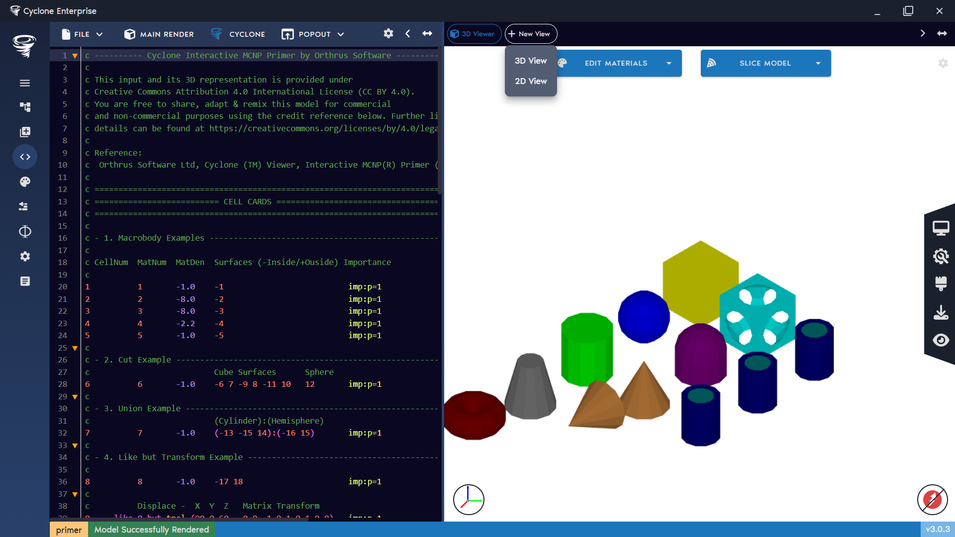
Figure 50: New 2D/3D view in main viewer

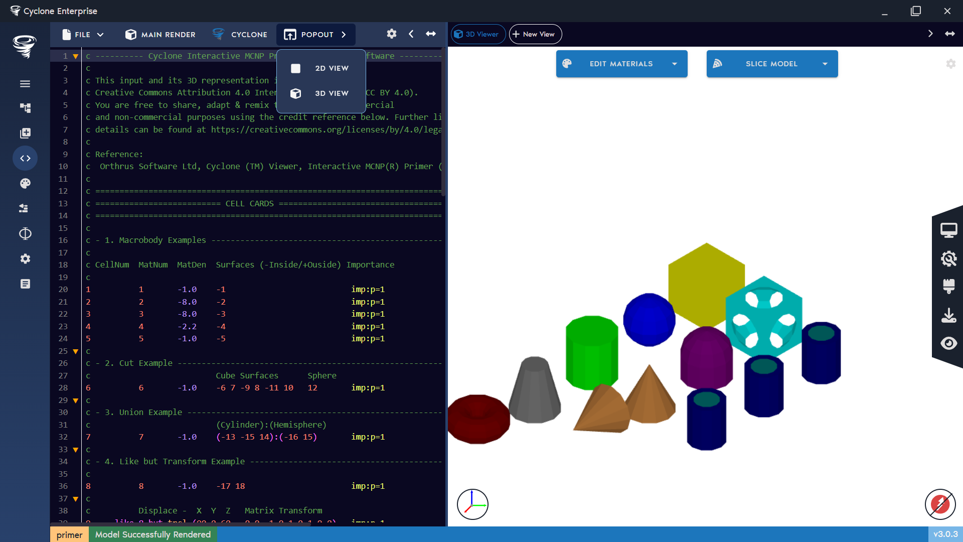
Figure 51: New 2D/3D view in popout window

Figure 52: Main 2D view

Figure 53: 2D view – main sections highlighted

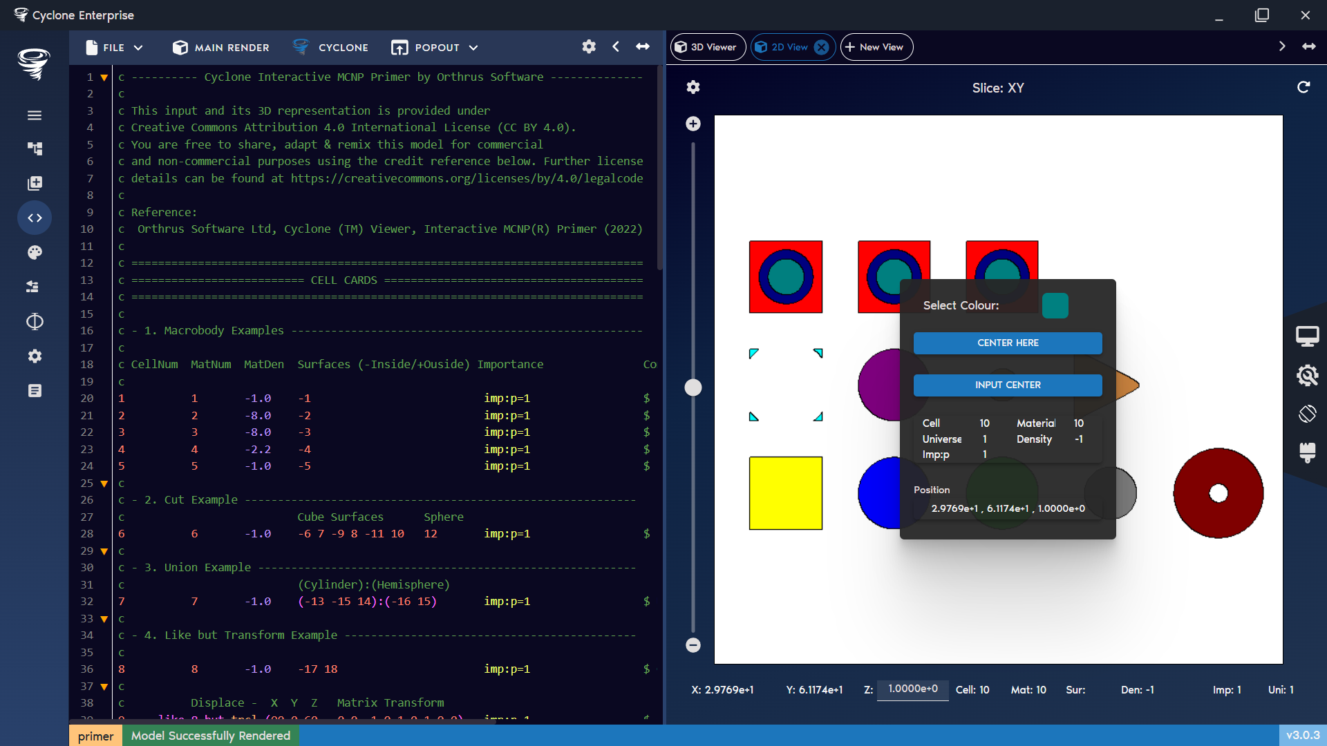
Figure 54: 2D view – context manu

Figure 55: 2D view – side menu

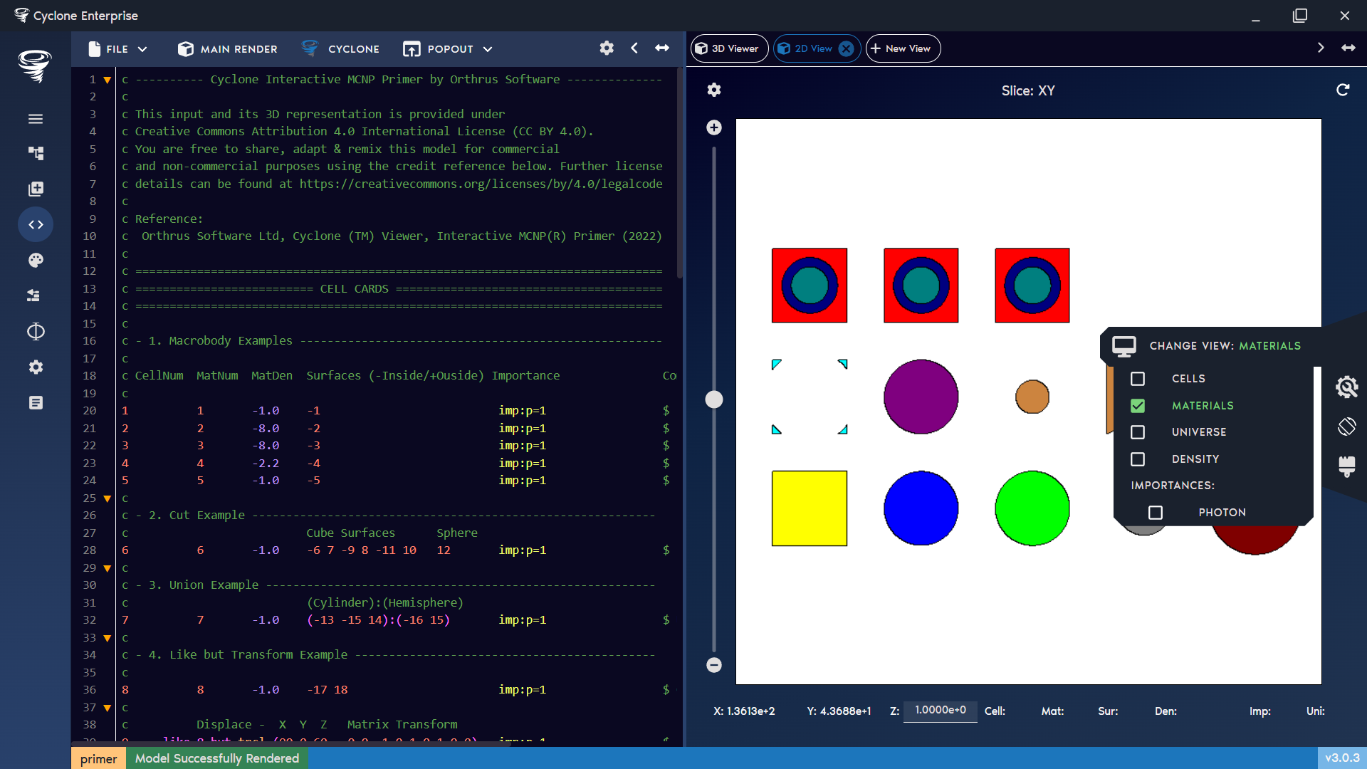
Figure 56: 2D view – change view preference

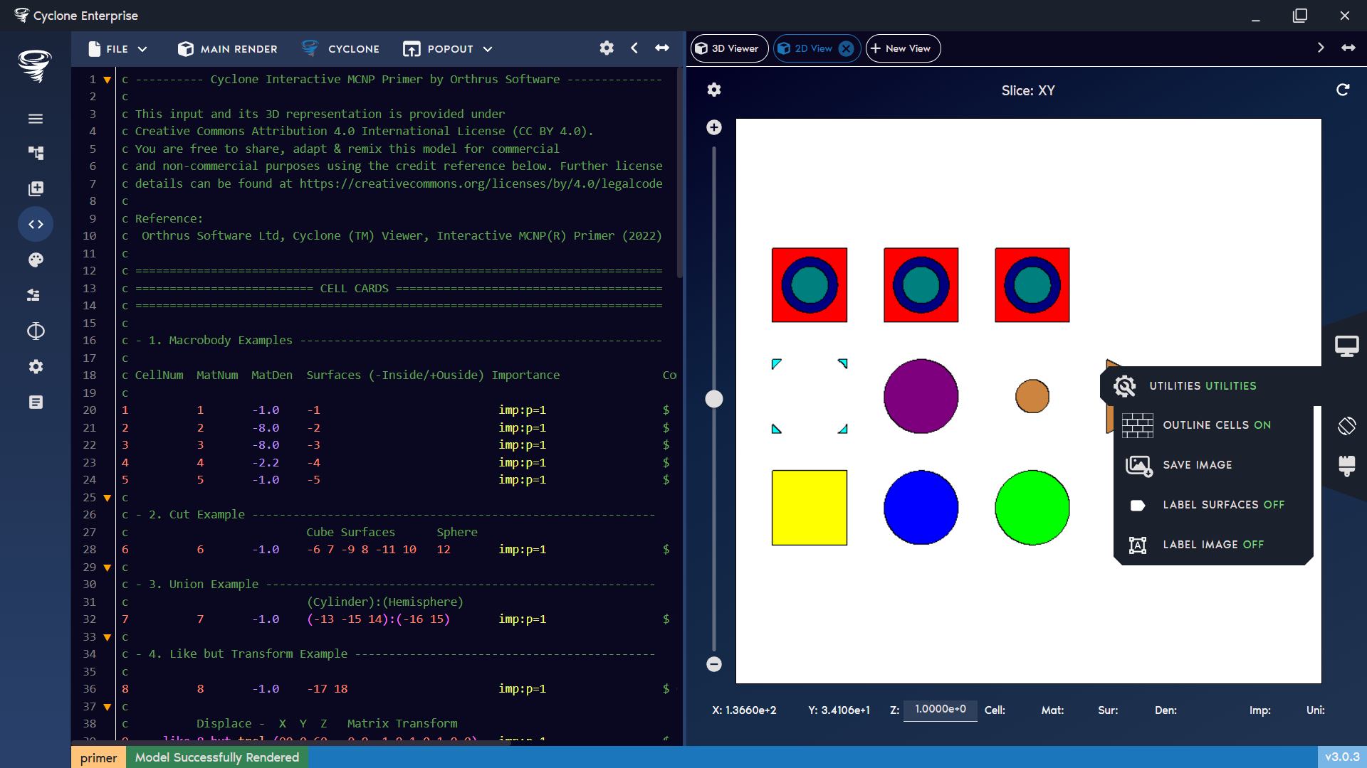
Figure 57: 2D view – utilities menu

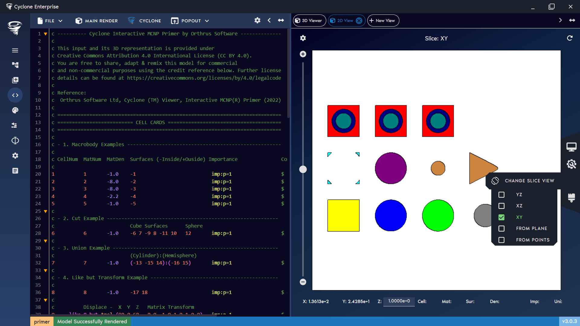
Figure 58: 2D view – change slice view

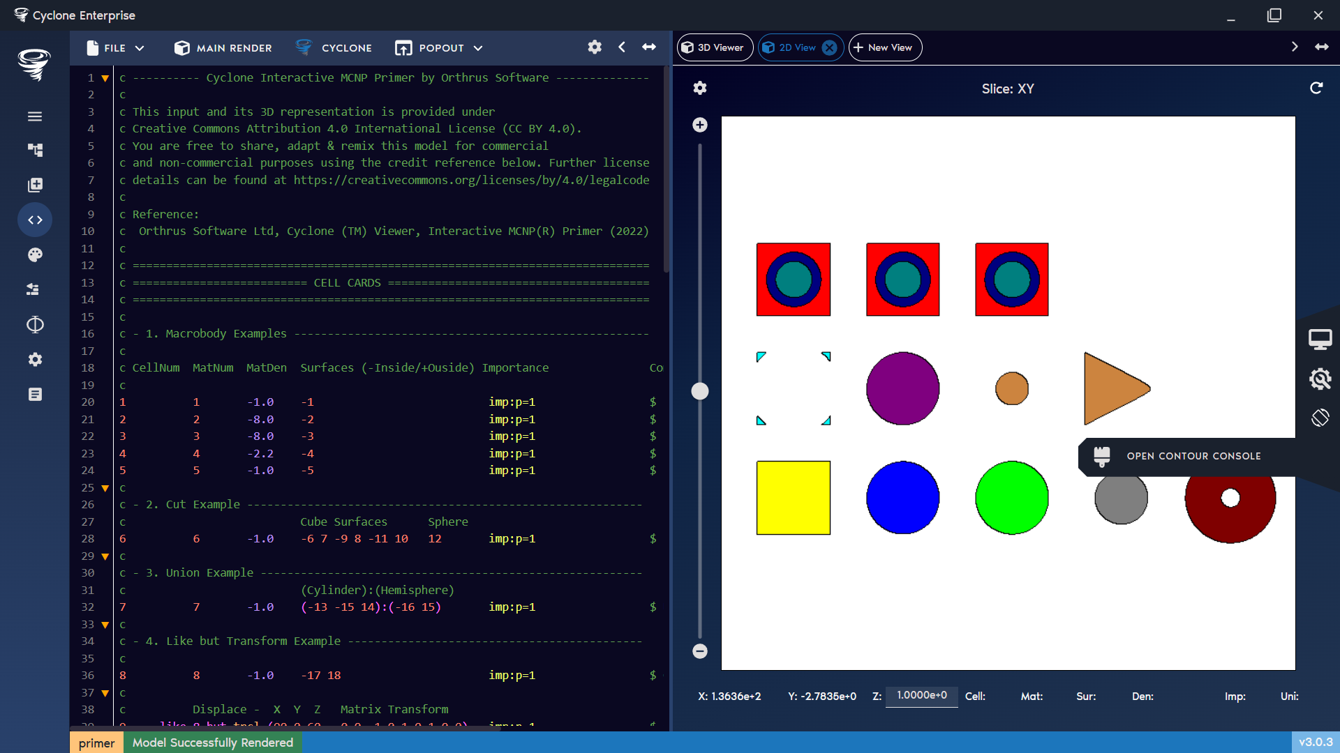
Figure 59: 2D view – open contours console

Figure 60: 2D view – zoom bar

Figure 61: 2D view – info bar

Figure 62: 2D view – settings cog

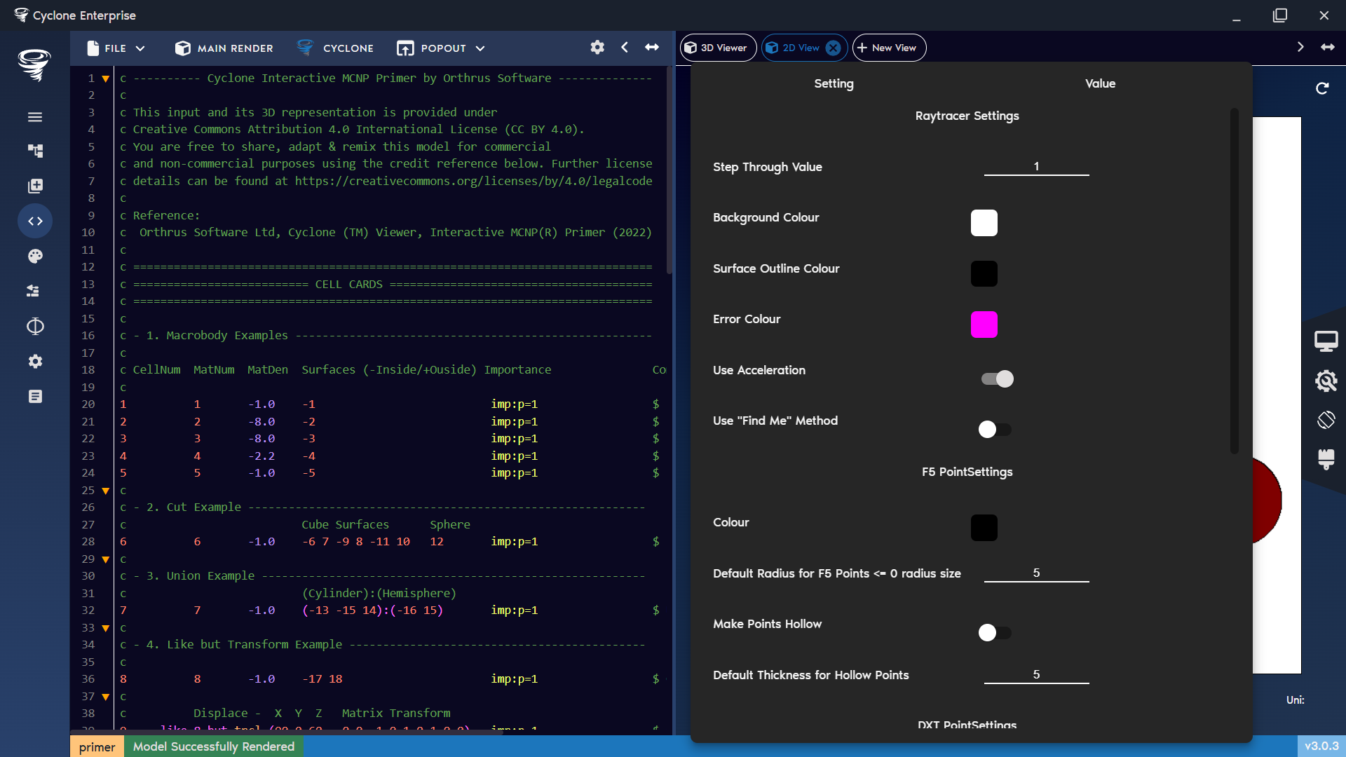
Figure 63: 2D view – settings menu

Figure 64: 2D view – refresh button

Figure 65: 2D view – draw box

Figure 66: 2D view – draw line

Table 6: 2D View Settings | Option | Description | |-------------------------------------|----------------------------------------------------------------------------------------------| | Step through value | Default value to step through the model with the mouse wheel. | | Background Colour | Set the background colour of the view. | | Surface Outline Colour | Set the colour of the surface outlines. | | Error Colour | Set the colour used to highlight overlaps and voids. | | Use Acceleration | Enable acceleration structures to improve raytracer performance. | | Use “Find Me” Method | Switch the view mode from default to using the “find me” function. | | Ambient Light Amount | Adjust the strength of ambient lighting. | | Diffuse Light Amount | Adjust the strength of diffuse lighting. | | F5 PointSettings | | | Colour | Set the colour of F5 point tallies. | | Default Radius for F5 Points ≤ 0 | Set the default radius for F5 point tallies when their defined radius is 0 or less. | | Make Points Hollow | Display F5 points as hollow rings instead of solid spheres. | | Default Thickness for Hollow Points | Set the default thickness of hollow F5 points. | | DXT PointSettings | | | Colour | Set the colour of DXT points. | | Default Radius for DXT Points | Set the default radius for DXT spheres. | | Make Points Hollow | Display DXT points as hollow rings instead of solid spheres (useful for nested DXT spheres). | | Default Thickness for Hollow Points | Set the default thickness of hollow DXT points. | | KSRC PointSettings | | | Colour | Set the colour of KSRC points. | | Default Radius for KSRC Points | Set the default radius for KSRC points. | | Make Points Hollow | Display KSRC points as hollow rings instead of solid spheres. | | Default Thickness for Hollow Points | Set the default thickness of hollow KSRC points. |

Contour console

The Open Contour Consoles button from the side menu in the 2D/3D view opens the main contour widget (Figure 67). The default view opens on contours. The user can switch between Contours, Particle Tracks, CAD (3D only) and the Live View widgets from the top menu (Figure 68).

Plotting Mesh Tallies

A mesh tally can be loaded into cyclone with the Import Mesh Tally button. Once loaded it will appear in the list of mesh tallies. The user can select a mesh tally and create a contour from it, an isosurface or map the contour to surfaces in the 3D view. Mesh tallies can be combined using the calculator.

Loading Mesh Tallies

The first button is the Import button (Figure 69). Clicking on this will bring up the import file box (Figure 71). The user should navigate to the mesh tally file they wish to import and click open. Once imported the mesh tally will appear in the table (Figure 70).

Supported Mesh Tally Types

Cyclone supports the following mesh tally output formats:

• Rectilinear mesh tallies where out = col, colsci, cf, cfsci, ij, ik, jk, xdmf.

• Note: For out = xdmf, Cyclone does not require the XDMF file itself—it only reads the runtape file that is generated.

• CSV format, which can be used for user-created files (rectilinear only).

Mesh Tally CSV File Format

The CSV file describes one or more mesh tallies.

Each file is divided into tally blocks, and each block begins with a TALLY marker line.

File Structure:

HTML
Copy
1TALLY,<shape>
2<name>,<x>,<y>,<z>,<flux>,<error>
3<name>,<x>,<y>,<z>,<flux>,<error>
4...
5TALLY,<shape>
6<name>,<x>,<y>,<z>,<flux>,<error>
7...

• Each TALLY line marks the start of a new tally block.

• Each block contains data lines with the tally values.

The TALLY Marker Line:

HTML
Copy
1TALLY,<shape>

• TALLY (case-insensitive) is mandatory.

• <shape> defines the mesh shape:

• "R" → Rectangular grid

• Anything else (or omitted) → Non-rectangular grid

When a new TALLY line is read, the previous block (if any) is finalized, and a new tally begins.

Data Lines:

Each data line defines one voxel value in the tally:

HTML
Copy
1<name>,<x>,<y>,<z>,<flux>,<error>

• <name> – Name of the tally (string, must be the same across all rows in a block).

• <x>,<y>,<z> – Coordinates of the mesh point (numbers, may be floats).

• <flux> – Flux value at this point (float).

• <error> – Relative error or uncertainty (float).

All coordinates are collected into sorted unique sets (xMidPoints, yMidPoints, zMidPoints).

Flux/error values are placed into a 3D array indexed by (x,y,z).

Example:

Below is a valid CSV with two tallies:

Plain text
Copy
1TALLY,R
2flux1,0.0,0.0,0.0,1.23,0.05
3flux1,1.0,0.0,0.0,1.10,0.04
4flux1,0.0,1.0,0.0,1.15,0.06
5flux1,1.0,1.0,0.0,1.05,0.03
6TALLY,CYL
7flux2,0.0,0.0,0.0,2.50,0.07
8flux2,0.0,0.0,1.0,2.45,0.08
9flux2,0.0,1.0,0.0,2.60,0.06
10flux2,1.0,0.0,0.0,2.55,0.07

• First block: a rectangular grid tally (shape = R) named flux1.

• Second block: a non-rectangular grid tally (shape = NR).

Rules and Notes:

• One tally per block. All rows until the next TALLY line belong to the same tally.

• Consistent naming. Within a block, <name> must be identical.

• Complete grids. All combinations of X, Y, Z that define the mesh must be provided. Missing points will cause indexing errors.

• Multiple tallies. Just add more TALLY blocks in sequence.

Common Pitfalls:

• Forgetting the TALLY line before the first block (the reader won’t know a new tally has started).

• Inconsistent names inside one block.

• Missing coordinate triplets → causes Indexing error in CSV reader.

Future Development

We are actively working on supporting more formats including cylindrical and spherical geometry.

Exporting Mesh Tallies

Clicking on export, exports the active mesh tally in a CSV format.

Creating Mesh Tallies

New mesh tallies can be created from existing mesh tallies using the mesh tally calculator (Figure 72). The user can combine mesh tally data, scale, and perform other mathematical functions on them. If performing an operation between two mesh tallies, they must share a common mesh, i.e. the mesh when fully expanded needs to be the same in both mesh tallies.

Once saved the mesh tally will appear in the mesh tally list. All available operations are shown in Table 7.

Caching

Mesh tallies when read or created are timestamped and cached into a database file. If the mesh tally is updated, cyclone checks the time stamp and will reread and reload the data if the mesh tally is found to be newer, otherwise is loads the data from the cached database file.

Creating a Contour

Selecting the Create Contour widget opens a set of options for plotting contour data.

• In the 3D view, the user can define a plane on which to plot the contour (Figure 73).

• In the 2D view, the contour is plotted directly on the current slice plane (Figure 74).

Available options include:

• Choosing the tally to plot.

• Selecting the data type (result or error).

• Applying a scaling factor.

• Choosing a colour scheme to map the results.

Click + Contour to add the contour to the active 2D or 3D view. Once added, it will appear in the Live View widget list.

Creating an Isosurface (3D view only)

In the 3D view, isosurfaces can be generated at a specified value (Figure 75). Adjust the extraction value, then click + Isosurface to add it to the view. Once created, the isosurface will appear in the Live View widget list.

Creating a Surface Contour (3D view only)

A mesh tally can be mapped onto a surface, or a group of surfaces, using the Create Surface Contour option (Figure 76). Mapping can be applied to selected cells, materials, or to CAD models that have been loaded into the view through the Overlay CAD Section 16.4.3. Once created, the contour will appear in the Live View widget list.

Plotting Particle Tracks

Similar to mesh tallies, a particle track file can be uploaded into Cyclone. Supported formats include ASCII, binary, and HDF5 particle track files.

To import:

• Select Import ptrack file.

• Navigate to the file and click Open.

As with mesh tallies, Cyclone creates a database file to cache the data, along with a timestamp. If a newer version of the particle track file is detected, the cached data is invalidated and replaced with the updated version; otherwise, the cached data is used.

Click ADD to add the particle track file to the Live View widget list, Figure 77.

Overlay CAD (3D View Only)

CAD files can be imported and overlaid into the 3D view (Figure 78). Supported file formats are STL, OBJ, IGS, and STP. For IGS and STP files, an import resolution is applied during loading.

To import a CAD file:

• Select Import CAD File.

• Navigate to the desired file and click Open.

• Once the file appears in the table, click ADD to include it in the Live View widget list.

Live View Widget

Anything that gets added to the current 2D/3D view appears in the Live View widget. Here the user can select the view, turn it on/off, delete it, or change the settings of the live view, different options are available depending on the type of live view, i.e. contour, isosurface, particle tracks, etc. See Figure 79.

Contours

Contour settings can be adjusted quickly (Figure 80), including the scaling factor, display type, slice plane, and position in space.

The appearance of the contour is highly configurable:

• The slice axis can be changed and the position in space can be moved.

• Data can be shown as raw voxelised values or interpolated from 3D data.

• Colours can be displayed in bands or smoothly interpolated.

• Colour schemes can be customised and normalised to different data ranges.

• Opacity can be adjusted to control contour visibility.

• A colour scheme key can be created from the current contour and added to the live view.

Examples shown in Figure 81.

Isosurfaces

Isosurface settings (Figure 82) can be adjusted quickly, including the scaling factor and the extraction value.

The colour of the isosurface is highly configurable:

• Colours can be displayed in bands or smoothly interpolated.

• Colour schemes can be customised and normalised to different data ranges.

• Opacity can be adjusted to control isosurface visibility.

• A colour scheme key can be created from the current contour and added to the live view.

Examples shown in Figure 84.

Surface Contours

Surface contours have similar settings to regular contours (Figure 83). They can be adjusted quickly, including the scaling factor, display type and colour scheme.

The appearance of the surface contour is highly configurable:

• Data can be shown as raw voxelised values or interpolated from 3D data.

• Colours can be displayed in bands or smoothly interpolated.

• Colour schemes can be customised and normalised to different data ranges.

• Opacity can be adjusted to control contour visibility.

• A colour scheme key can be created from the current surface contour and added to the live view.

Examples shown in Figure 85.

Particle Tracks

Particle track settings can be adjusted quickly (Figure 86), colours can be changed^3 and the amount of particles to show can be changed or turned on/off.

• Colours can be changed from block to interpolated over any colour scheme.

• Source particles can be turned on/off and the amount to show can be changed.

• Particle collisions can be turned on/off and the amount to show can be changed.

• Particle Tracks can be turned on/off and the amount to show can be changed.

• A colour scheme key can be created from the current contour and added to the live view.

CAD

Imported CAD models can be adjusted in the view using simple transforms (Figure 87), allowing them to be scaled, translated, or rotated in place. For more complex transformations, a full 4×4 transformation matrix can be applied instead (Figure 88).

Colour Keys

For most views that use colour schemes, a colour key can be generated. The key can be customised in terms of appearance, layout, precision, name, and colour, and it can be freely dragged to any position on the image.

A colour key can either be isolated (independent of the view that created it) or linked so that it automatically updates whenever the corresponding view is updated. See Figure 89.

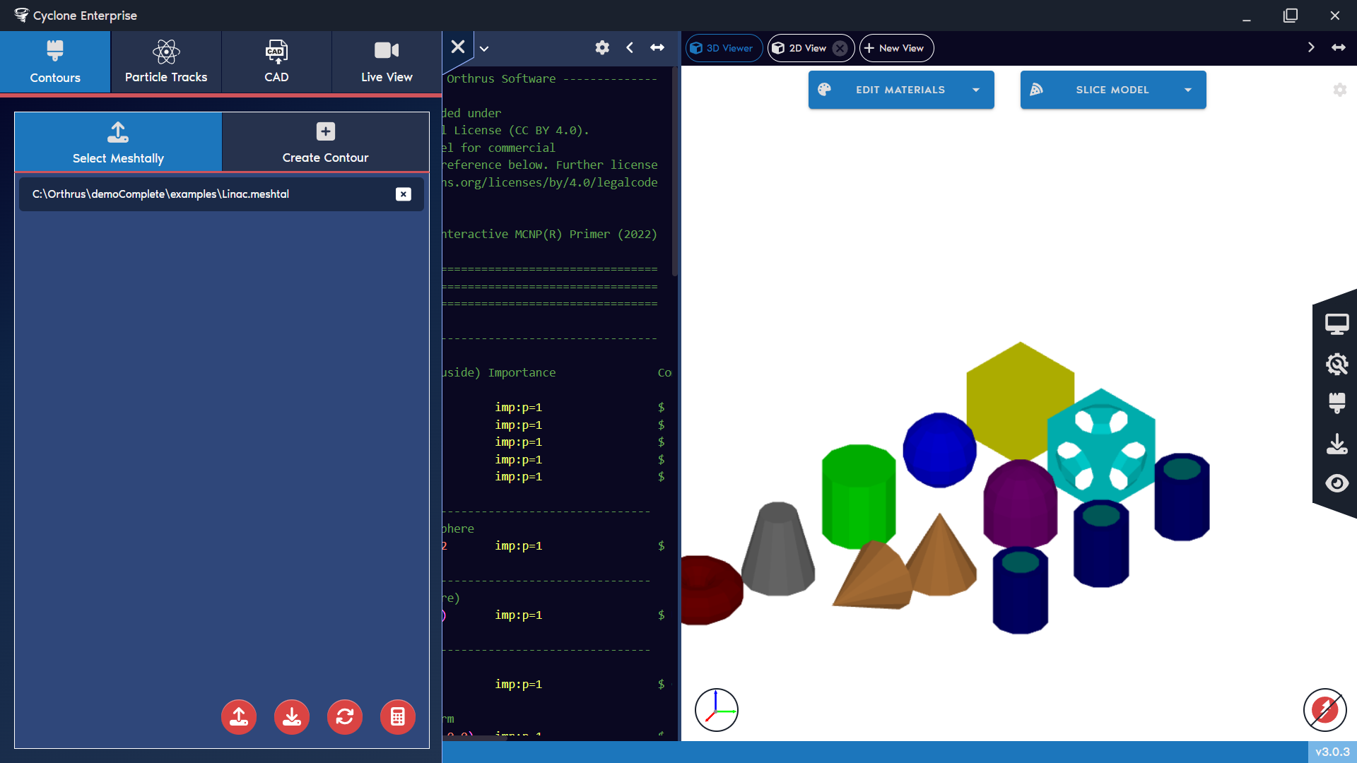
Figure 67: Contour console overview

Figure 68: Contour console – switch between widgets

Figure 69: Contour console – mesh tally operations

Figure 70: Contour console – select mesh tally

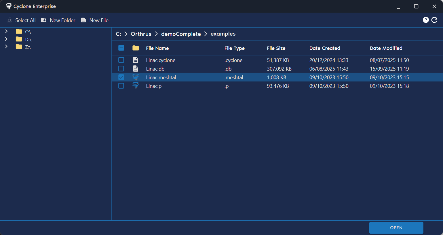
Figure 71: Contour console – import mesh tally

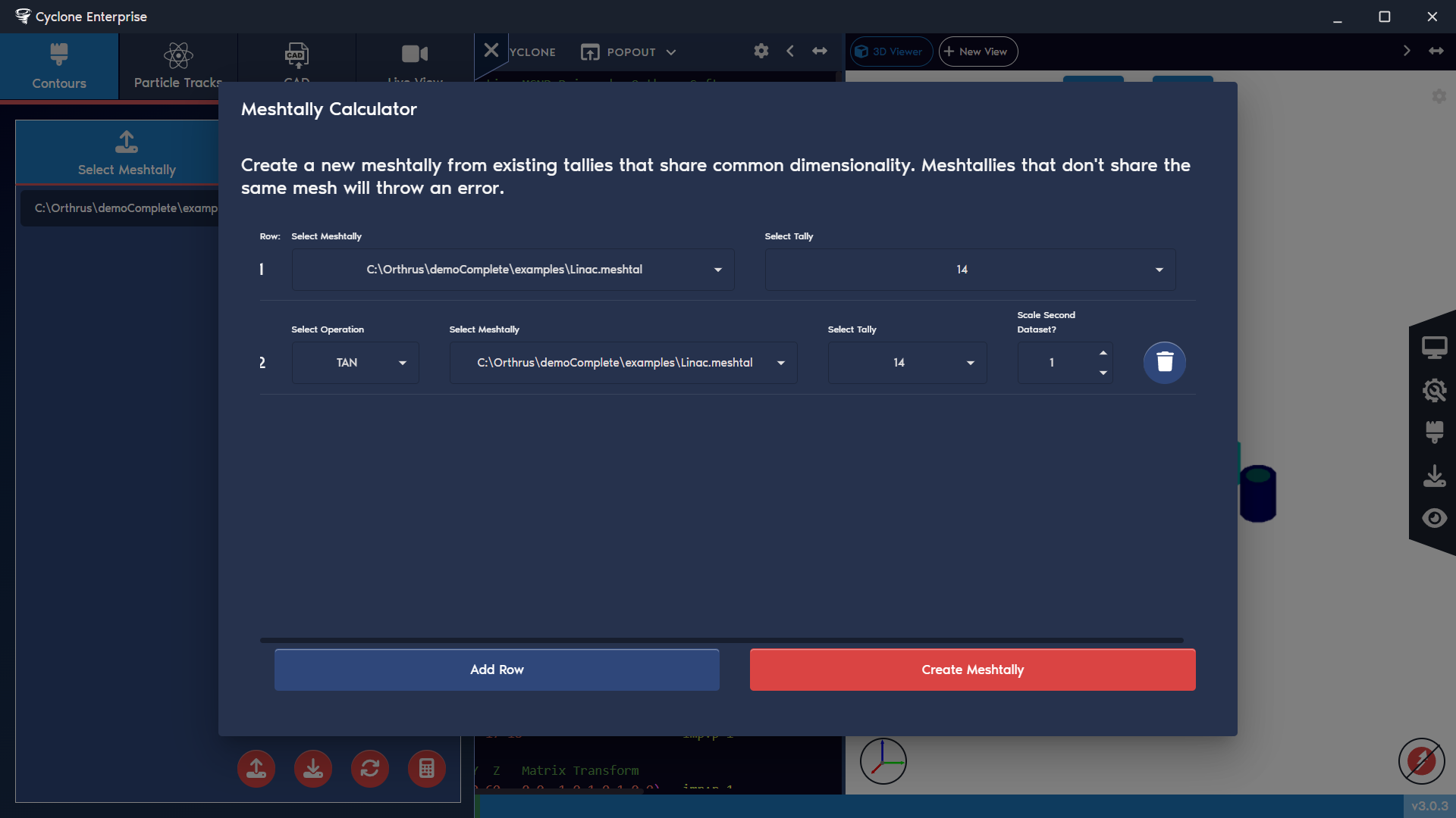
Figure 72: Contour console – mesh tally calculator

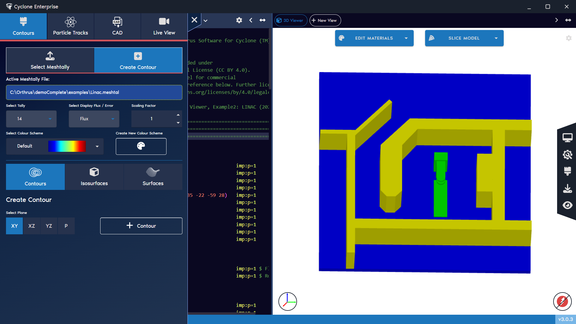
Figure 73: Contour console – create contour 3D view

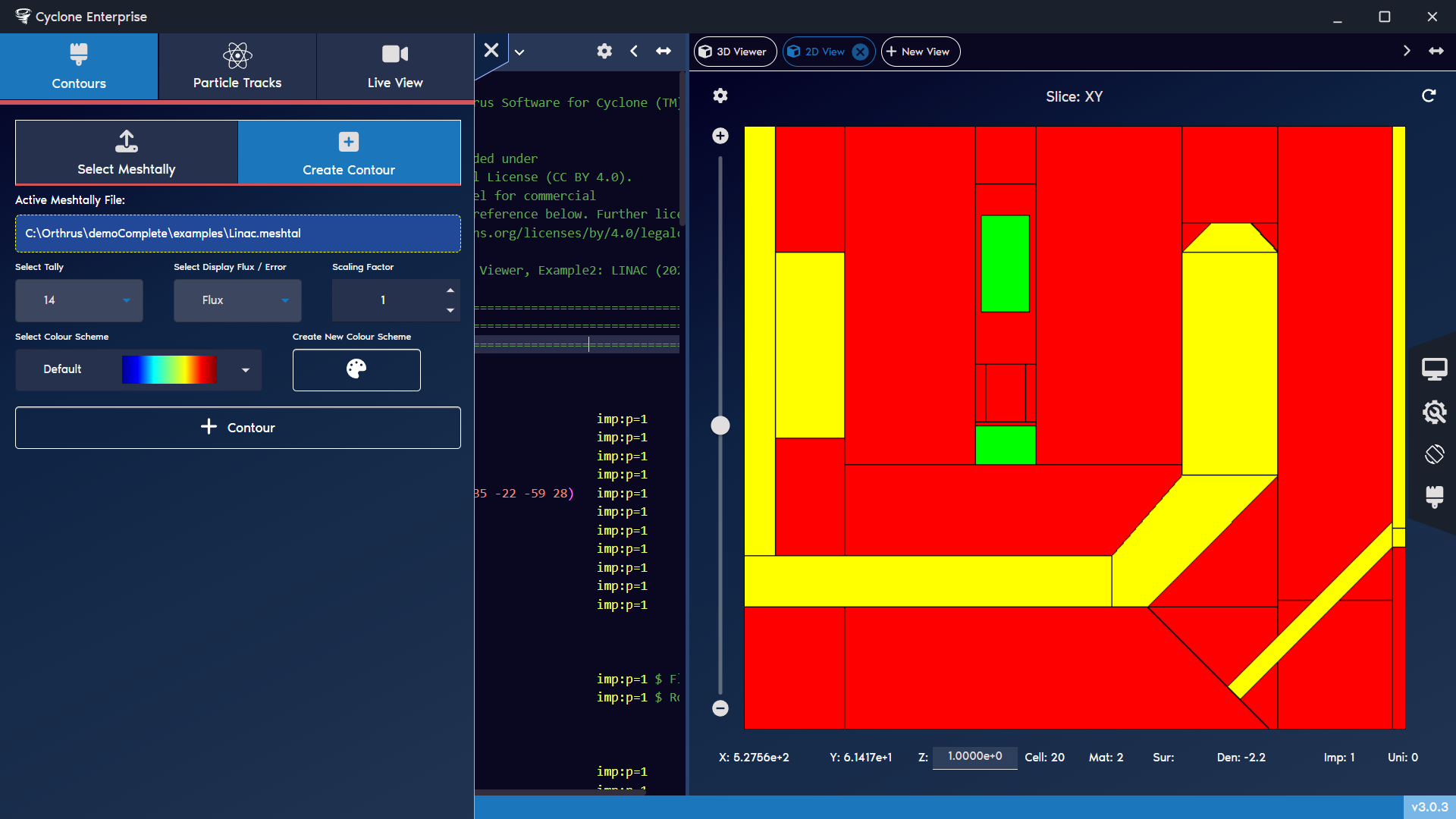
Figure 74: Contour console – create contour 2D view

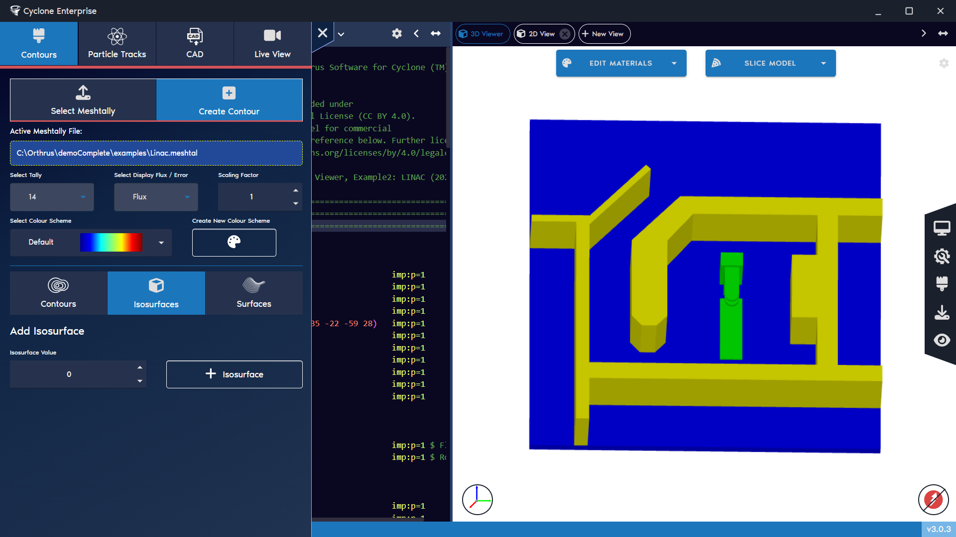
Figure 75: Contour console – create isosurface

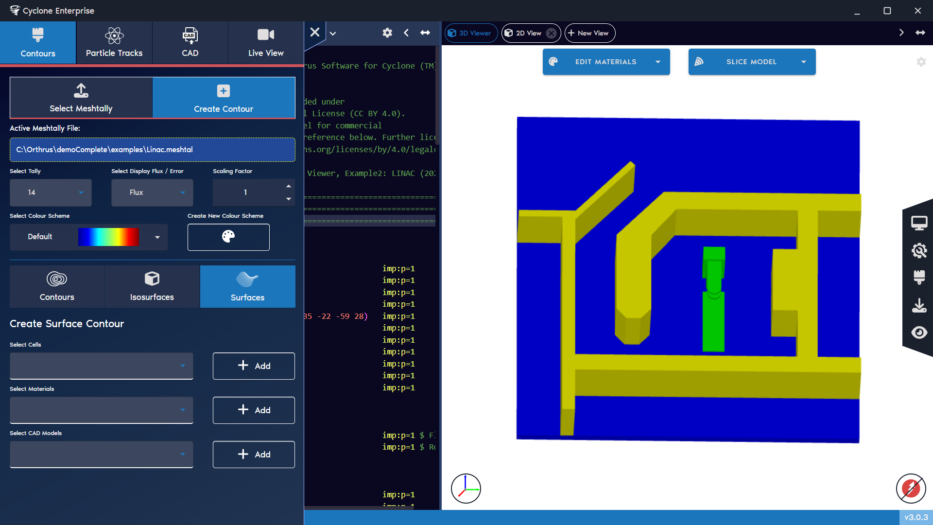
Figure 76: Contour console – create surface contour

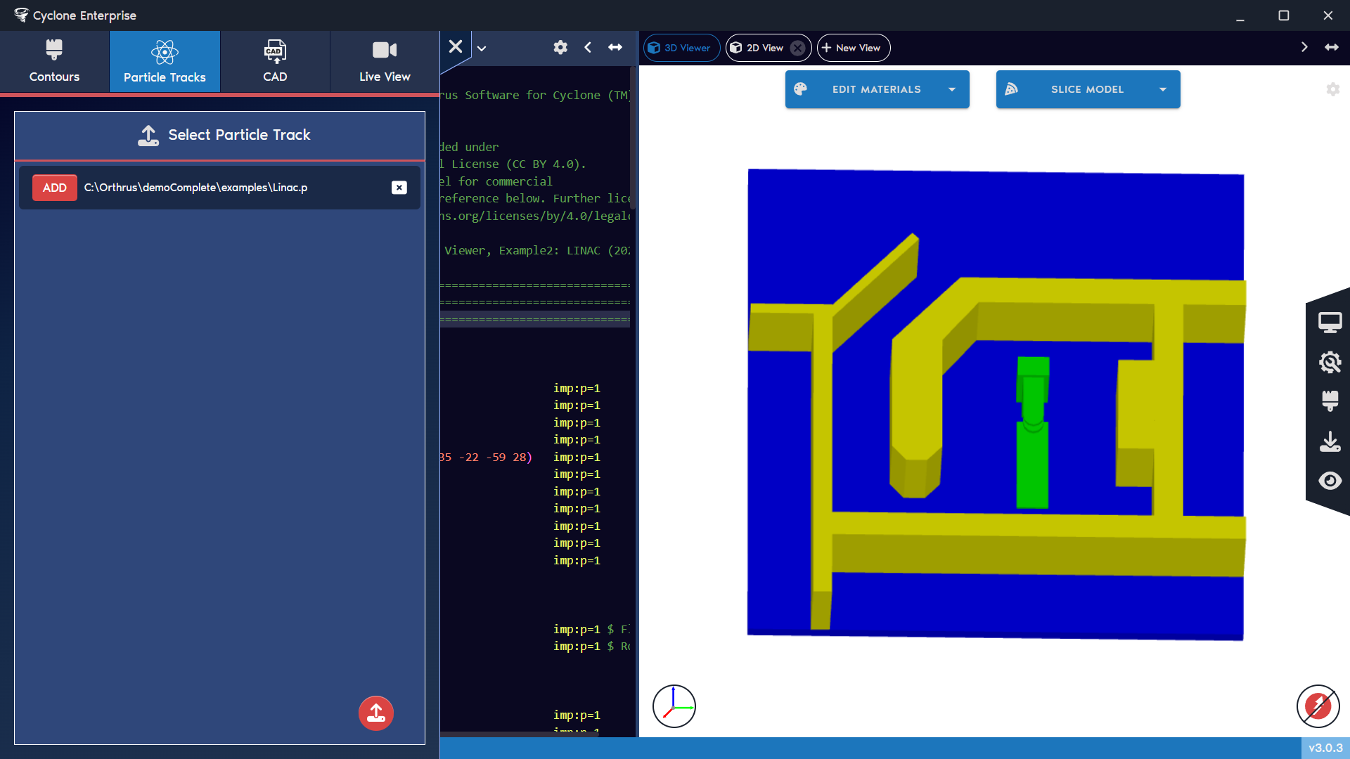
Figure 77: Contour console – particle tracks

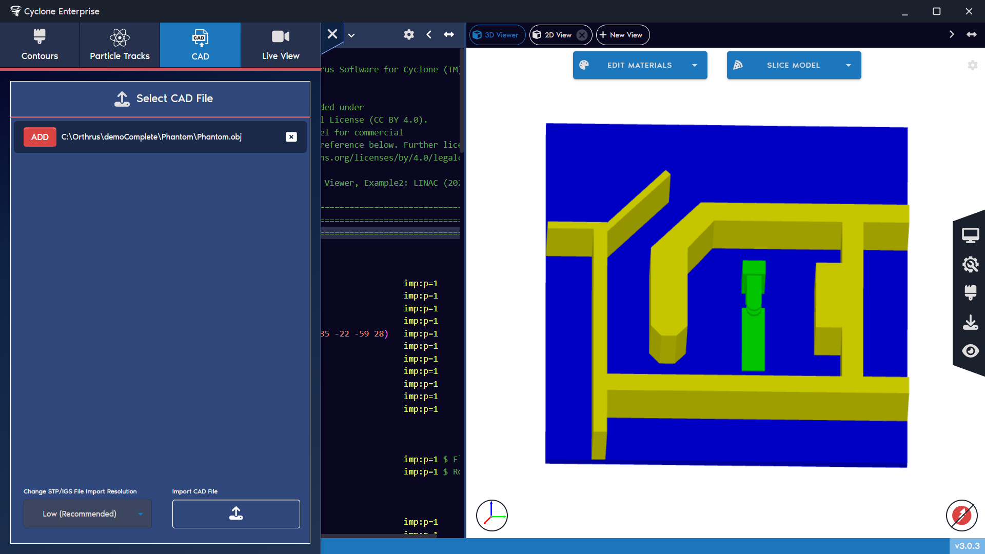
Figure 78: Contour console – CAD

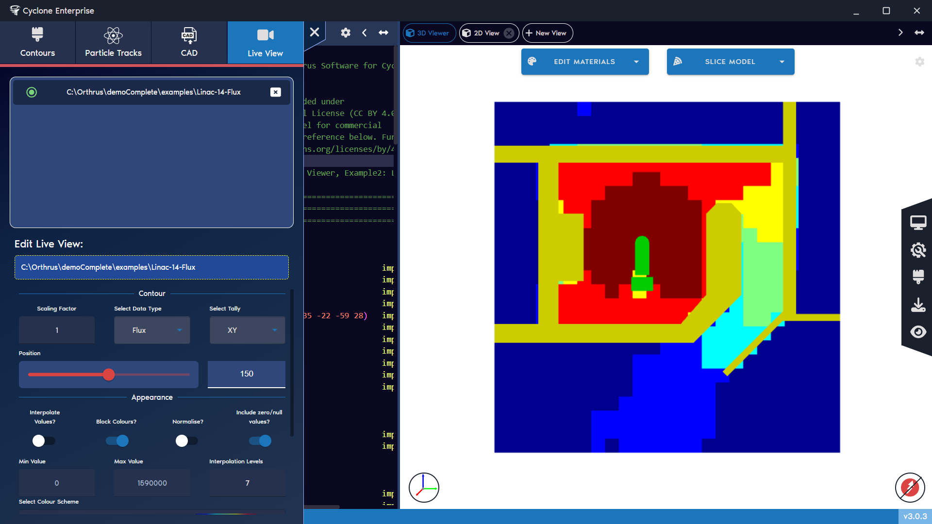
Figure 79: Contour console – live views

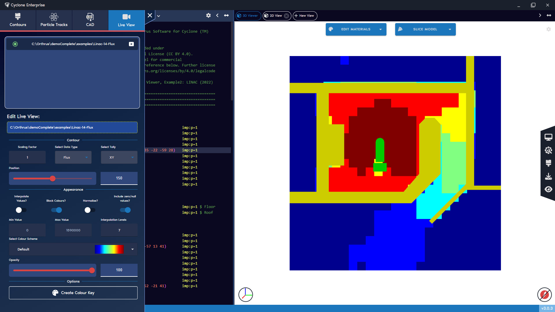
Figure 80: Live views – contour options

Figure 81: Contours, top left (banded colours, voxelised data); top right (banded colours, interpolated data); bottom right (interpolated colours, voxelised data); bottom right (interpolated colours, interpolated data)

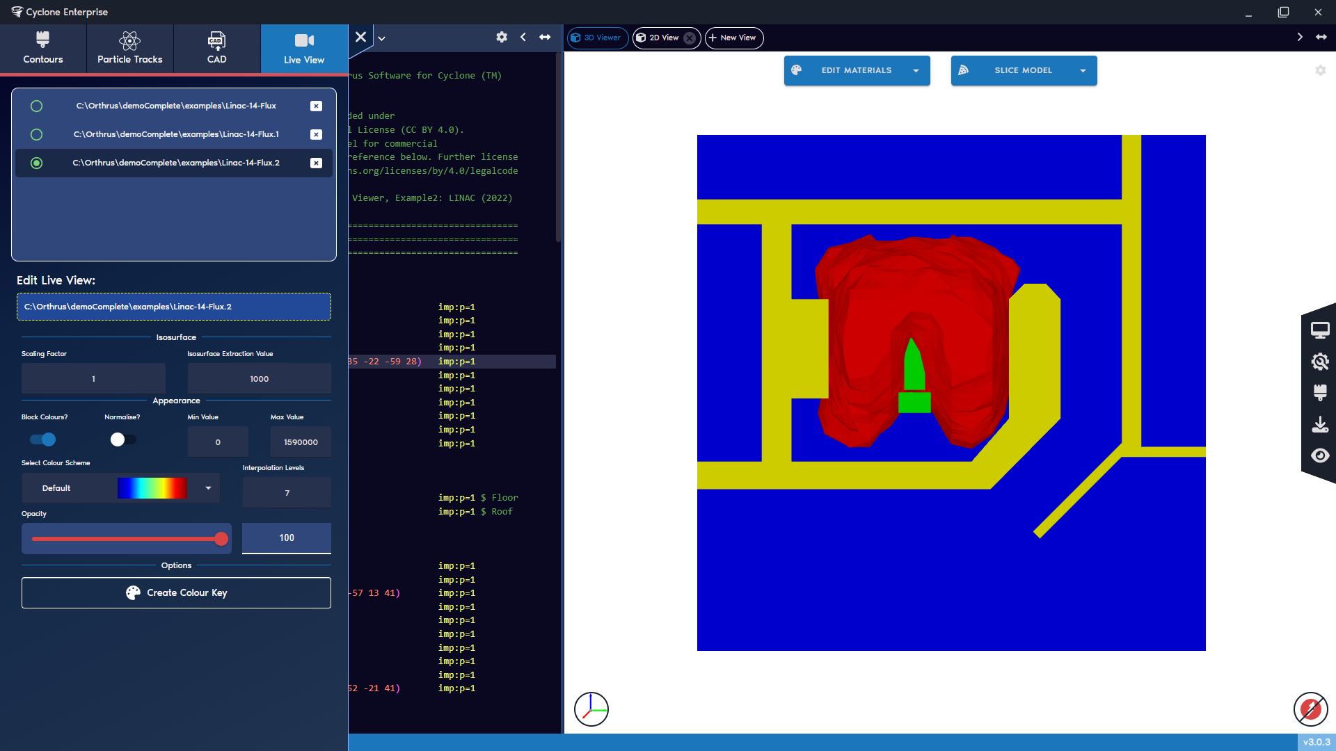
Figure 82: Live views – isosurface options

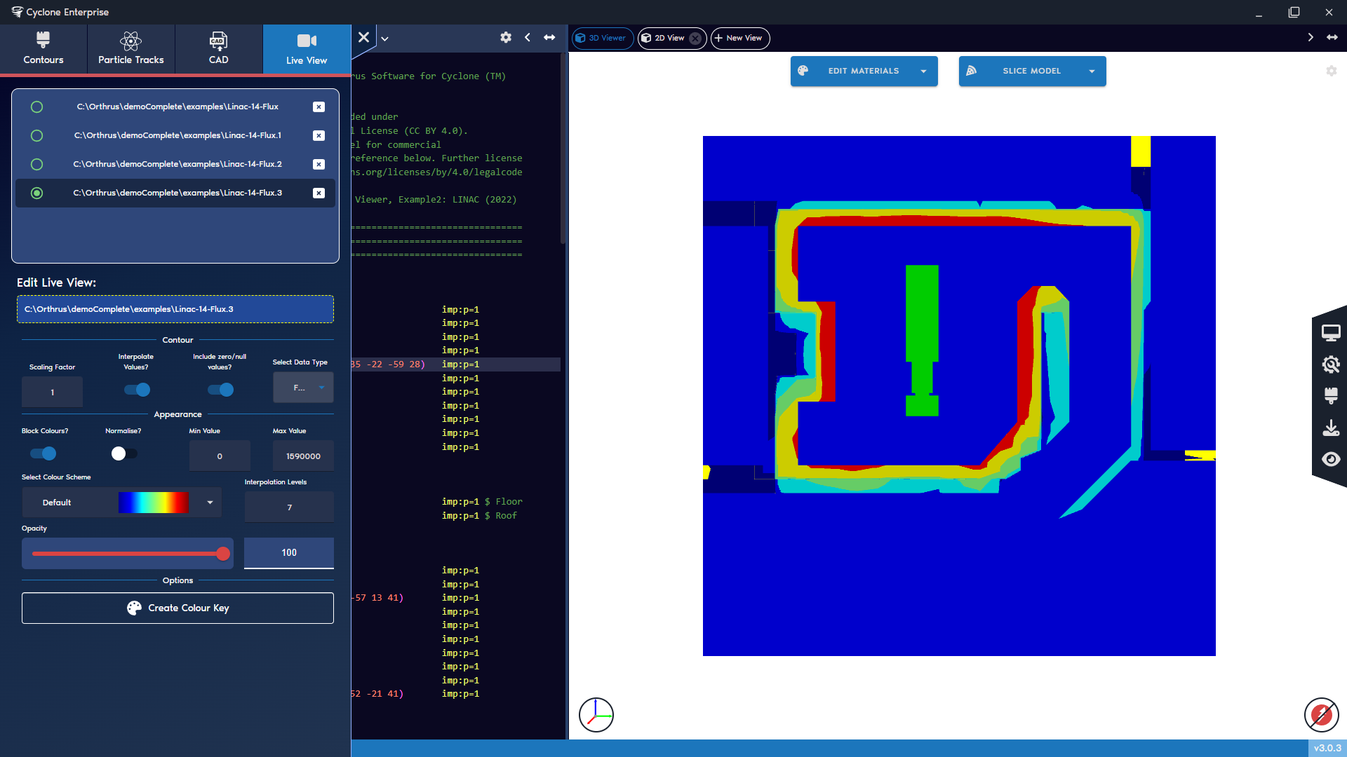
Figure 83: Live views – surface contour options

Figure 84: Isosurface extraction values at 10000 (top left), 1000(top right), 100(bottom left) and 10(bottom right)

Figure 85: Surface contours, top left (banded colours, voxelised data),top right (banded colours, interpolated data), bottom right (interpolated colours, voxelised data), bottom right (interpolated colours, interpolated data)

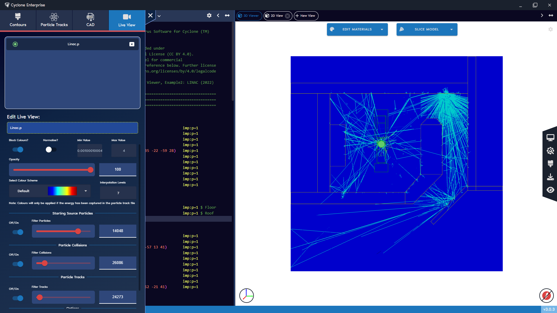
Figure 86: Live views – particle tracks

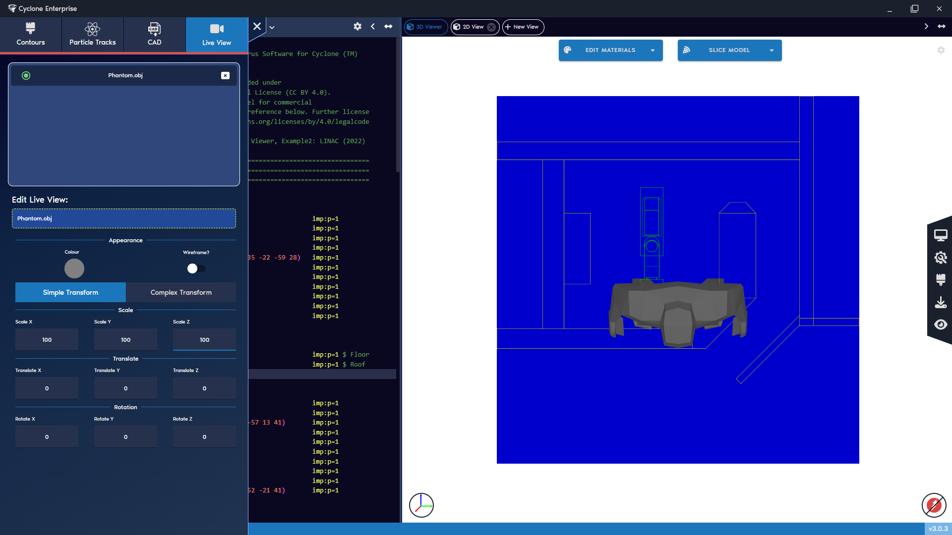
Figure 87: Live views – CAD simple transformation

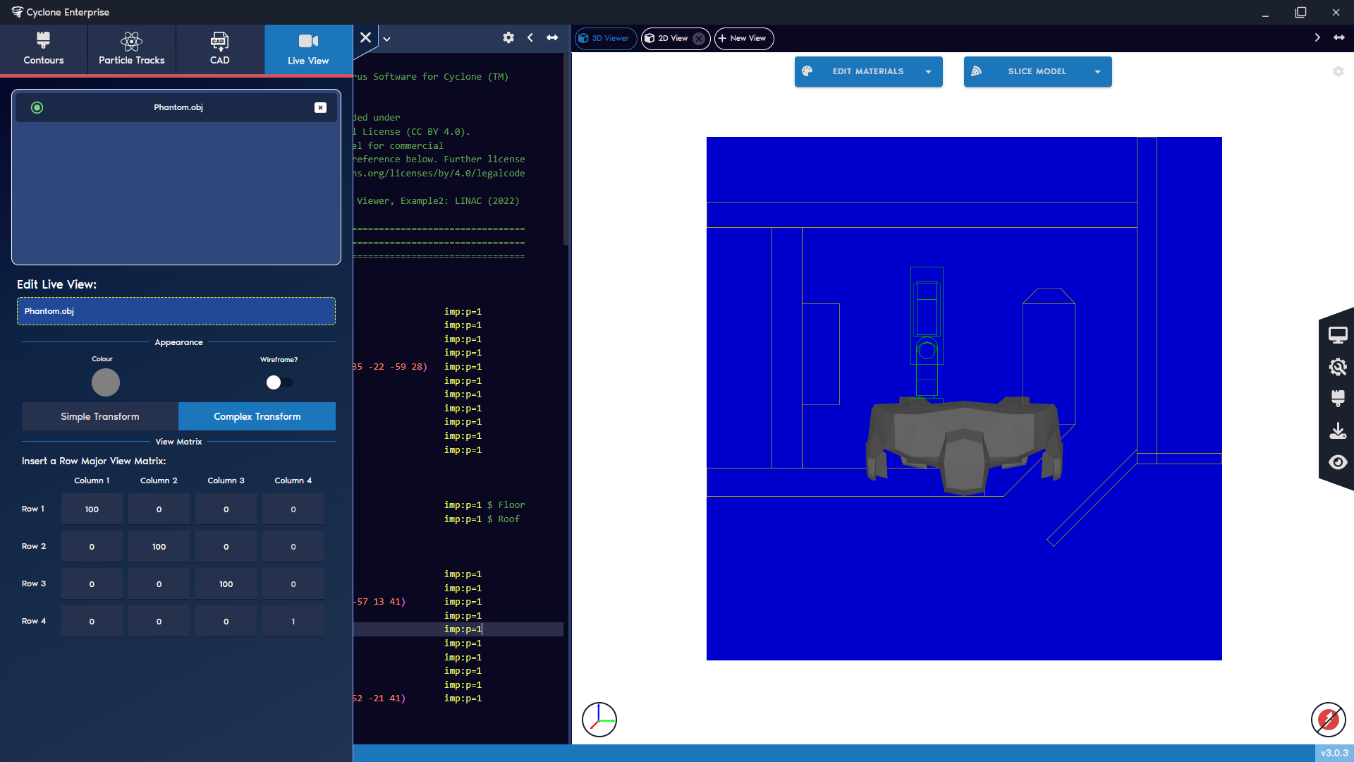
Figure 88: Live views – CAD complex transformation

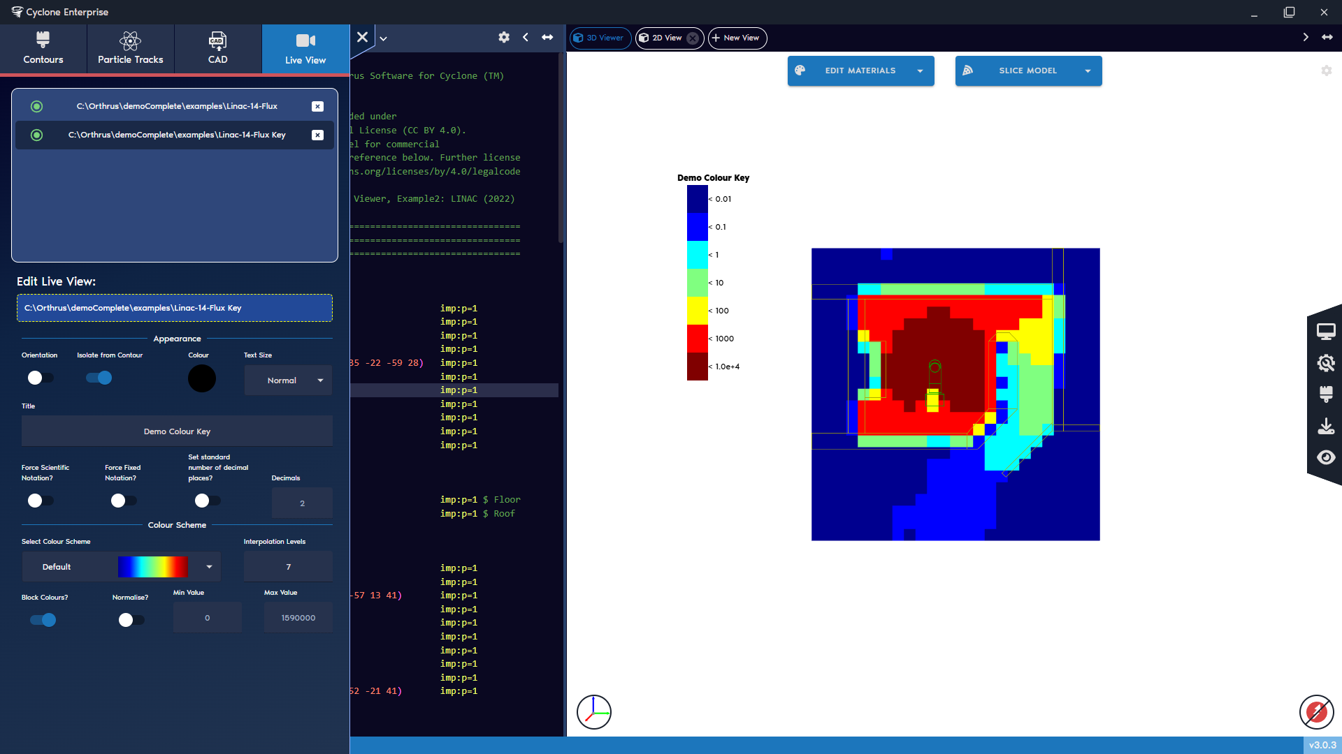
Figure 89: Live views – colour keys

Table 7: Mesh tally Calculator Operations